Why it matters
The simple sorts from lesson 1 do about n squared steps. For a list of a million values, that is about a trillion steps, which takes a long time even on a fast computer. Merge sort and quick sort do about n log n steps. For a million values, log2 of n is about 20, so the work is about 20 million steps. That is roughly fifty thousand times less work, and it is the difference between a program that finishes and one that does not.
Both sorts use the same big idea. They break the problem into smaller problems of the same kind, solve the smaller ones, then combine the answers. That idea is called divide and conquer. Once you can write it, you can write many other fast algorithms, including binary search trees, the fast Fourier transform and most of the recursive solutions in the rest of this course. So this lesson is a good place to learn recursion properly.
Divide and conquer
Imagine a stack of five hundred exam papers that must be sorted by roll number. One person could do it alone, but it would take hours. A better plan is to split the pile in two, give each half to a helper, and ask each helper to sort their half the same way. When both halves come back sorted, you combine them into one sorted pile. The helpers use the same plan on their halves, so the splitting continues until a pile is so small that it is already sorted. A pile of one paper is always sorted.
A recursive function is a function that calls itself on a smaller input. The call that handles the smallest case is the base case. It stops the chain of calls. For sorting, the base case is an array with zero or one values, because such an array is already sorted and needs no work.
Recursion has one rule you must follow. Each call must make the input smaller, so that the base case is eventually reached. If a call does not shrink the input, it calls itself forever and the program crashes. The common mistakes section below shows what that crash looks like.
What happens inside a recursive call
When a function calls itself, the computer does not forget the first call. It stores the local variables of each call in a region of memory called the call stack. Each stored set of variables is a frame. A new frame goes on top when a call starts, and it is removed when that call returns. The top frame is always the one running.
For merge sort, the call on a big array waits while the call on its left half runs, then waits while the call on its right half runs. Then it does its own merge work and returns. At the deepest point, the stack holds one frame for each level of splitting. With a million values, the splitting goes about 20 levels deep, so the stack holds about 20 frames. That is small. The depth is what makes these algorithms safe to use on big inputs.
Merging two sorted piles
Merge sort depends on one simple operation: combining two sorted piles into one sorted pile. The method is easy. Look at the front card of each pile. Take the smaller one and put it on the output. Repeat until one pile is empty. Then copy the rest of the other pile.
Take two sorted piles, 27 38 and 3 43. Here is the merge, one step at a time.
- Compare the fronts, 27 and 3. Three is smaller, so take it. Output:
3. Left pile still starts with 27, and the right pile now starts with 43. - Compare 27 and 43. Twenty-seven is smaller, so take it. Output:
3 27. Left pile now starts with 38. - Compare 38 and 43. Thirty-eight is smaller, so take it. Output:
3 27 38. The left pile is now empty. - The left pile is empty, so copy the rest of the right pile, which is 43. Output:
3 27 38 43.
Four steps for four values. Each value was looked at once. Merging two piles of total size n always takes about n steps. That is the key fact for the speed of merge sort.
The merge code in the next section uses one more detail. When the two fronts are equal, it takes the value from the left pile first. That keeps equal values in their original order, which is what makes merge sort stable. You will see this in the code.
Merge sort
Merge sort is the sort that does the splitting and the merging. The algorithm is short:
- If the piece has zero or one values, stop. It is already sorted.
- Split the piece into a left half and a right half at the middle.
- Merge sort the left half. Merge sort the right half.
- Merge the two sorted halves back into the original piece.
Step 3 is the recursion. The two calls work on smaller pieces, so each call goes one level deeper. The splitting stops at pieces of size one, which take no work.
Tracing it on four values
Take the array 38 27 43 3. Here is the splitting and merging, with the call stack in mind. The program below prints each split and each merge, indented by depth, so you can match the trace.
Expected output:
split [38 27 43 3]
  split [38 27]
    split [38]
    split [27]
  merged [27 38]
  split [43 3]
    split [43]
    split [3]
  merged [3 43]
merged [3 27 38 43]
result: 3 27 38 43
Read the output from top to bottom. The first line is the whole array. The next line is the left half, 38 27. Its two single values are printed with no merge, because a single value is sorted. Then the left half is merged into 27 38. The right half, 43 3, goes through the same steps and becomes 3 43. The last merge combines 27 38 and 3 43 into 3 27 38 43, the same merge as in the previous section.
Outlined bars are being compared. Filled bars were just swapped or written. Bars with a dark border are in their final place. Faded bars are outside the part being worked on.
Split the list in halves, sort each half, then merge the halves.
Use the animation to watch the splits go down and the merges come back up. Look for two things. First, each merge only ever works on two sorted piles. Second, the widths of the piles double at each level going up, while the number of piles halves.
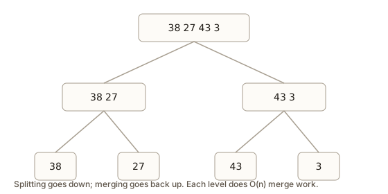 Merge sort tree for 38 27 43 3: the root splits into 38 27 and 43 3, which split again into single values, then merge back up to 3 27 38 43
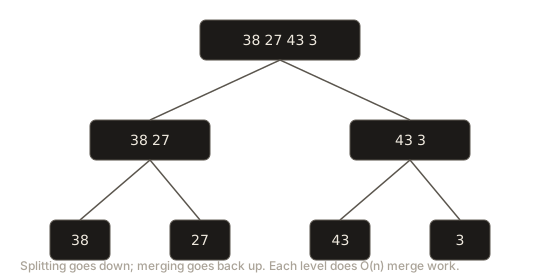
The picture shows the same tree. Going down is splitting, and coming back up is merging. Each level of the tree holds the whole array once, spread over more and smaller piles. That is the reason for the total work.
Why the work is n log n
There are about log2 n levels of splitting, because each split halves the size. A million values need about 20 levels, and a level is the set of pieces that are the same size. At each level, the merges together touch every value exactly once, which is about n steps. The total is the number of levels times the work per level, which is n times log n.
Merge sort is always this fast. Even a reversed or random array takes the same number of levels, because the split is by position, not by value. That is its great strength. It has no bad inputs.
The price is memory. The merge needs a place to put the merged output. The code below uses a temporary vector of the same size as the array, so the extra space is O(n). The sort is still fast, but it is not in place.
Merge sort code
The code below sorts an array with a temporary array for merging. It also counts inversions, which the next section explains. For now, notice the merge loop. It takes the left value when a[i] <= a[j], and the right value otherwise.
The program reads a count and then the numbers. Type these lines into the Input box:
6
3 1 2 5 4 0Expected output:
0 1 2 3 4 5
inversions: 8
Counting inversions with merge sort
An inversion is a pair of values that are out of order in the input. Two positions i and j with i < j form an inversion when the value at i is bigger than the value at j. For example, in 3 1 2, the pairs (3, 1), (3, 2) are inversions, and (1, 2) is not.
Inversions measure how far a list is from sorted. A sorted list has zero. A reversed list has the most, which is n times (n - 1) divided by 2. Bubble sort swaps exactly one inversion at a time, so the number of inversions is also the number of swaps bubble sort makes.
Counting inversions by checking every pair takes n squared steps. Merge sort can count them while it sorts, for free. The trick is in the merge. Suppose the left pile is sorted and the right pile is sorted. When a right value is smaller than the front of the left pile, it is smaller than every value still waiting in the left pile, because the left pile is sorted. So the right value forms an inversion with each of those waiting values. The count of waiting values is the number of values left in the left pile, which the code can read directly.
Here is the merge that counts. Look at the line inversions += mid - i + 1;. It runs only when the right value is smaller than the left front, and it adds the number of left values still waiting. The count is stored in a global variable, so every merge adds to the same total.
The program in the previous section printed inversions: 8 for the input 3 1 2 5 4 0. You can check that count by hand. The number 3 is bigger than 1, 2 and 0, which gives three inversions. The number 1 is bigger than 0, which gives one. The number 2 is bigger than 0, which gives one. The number 5 is bigger than 4 and 0, which gives two. The number 4 is bigger than 0, which gives one. The total is 3 + 1 + 1 + 2 + 1 = 8.
This technique is a common interview question. It answers "how far from sorted is this list?" in n log n time, instead of n squared. You will see it again when the question changes to counting pairs that satisfy some rule.
Quick sort
Quick sort takes a different route. Instead of splitting by position and merging afterwards, it splits by value. It picks one value called the pivot, rearranges the array so that every smaller value is on the left and every bigger value is on the right, and then sorts each side. After the rearrangement the pivot is already in its final place, because nothing on its left is bigger and nothing on its right is smaller.
Think of a class lining up by height. The teacher calls out a student of medium height. Everyone shorter moves to the left of that student, and everyone taller moves to the right. The chosen student is now in the right place for the final line. Now the two groups can be lined up by the same rule separately.
The rearranging step is called partition. This lesson uses a simple version called the Lomuto partition, which takes the last value as the pivot. It walks along the array with a pointer j, and it keeps a second pointer i that marks the boundary between the small values and the rest.
Partition step by step
Take the array 7 2 1 6 8 5 3 4. The pivot is the last value, 4. The boundary i starts at index 0, which means there are no small values yet. Walk j from index 0 to index 6, which is every position except the pivot.
- Look at 7, which is at
j= 0. It is not less than 4, so do nothing. The boundary stays at 0. - Look at 2, at
j= 1. It is less than 4. Swap it with the value at the boundary, which is 7. The array is2 7 1 6 8 5 3 4. Move the boundary to 1. - Look at 1, at
j= 2. It is less than 4. Swap it with the value at the boundary, which is 7. The array is2 1 7 6 8 5 3 4. Move the boundary to 2. - Look at 6, at
j= 3. It is not less than 4. Do nothing. - Look at 8, at
j= 4. Not less than 4. Do nothing. - Look at 5, at
j= 5. Not less than 4. Do nothing. - Look at 3, at
j= 6. It is less than 4. Swap it with the value at the boundary, which is 7. The array is2 1 3 6 8 5 7 4. Move the boundary to 3.
Now j has reached the pivot's position. The last step swaps the value at the boundary with the pivot. The boundary holds 6, so the array becomes 2 1 3 4 8 5 7 6. The pivot 4 sits at index 3, and everything to its left is smaller. Everything to its right is bigger.
The diagram below shows the array before and after this partition.
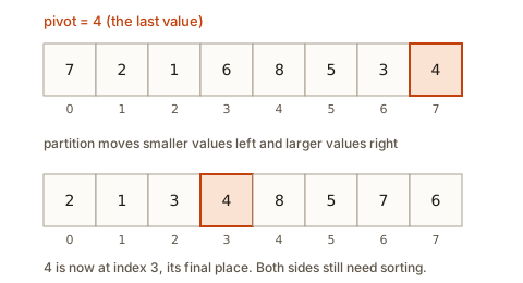 Two rows of eight boxes: before partition with pivot 4 at the end, and after partition with pivot 4 at index 3 and smaller values on its left
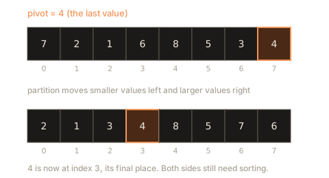
The part to the left of the pivot, 2 1 3, is not sorted yet, and neither is the part to the right, 8 5 7 6. Quick sort now calls itself on each side. Those calls do the same thing on their smaller pieces, and each call places its own pivot.
Outlined bars are being compared. Filled bars were just swapped or written. Bars with a dark border are in their final place. A triangle marks the pivot. Faded bars are outside the part being worked on.
Pick a pivot, move smaller items before it and larger after it, then repeat on each side.
Use the animation to watch the pivot land in its place and the sides shrink. The pivot is the value with the highlight, and the boundary is the pointer that moves right.
The quick sort code
The code below runs the Lomuto partition and prints the pivot and its final index for every partition call. It needs no input.
Expected output:
pivot 4 lands at index 3
  pivot 3 lands at index 2
    pivot 1 lands at index 0
  pivot 6 lands at index 5
    pivot 8 lands at index 7
1 2 3 4 5 6 7 8
The indentation shows the call depth. The top call places 4, and two calls below it place 3 and 6. Each of those places its own pivot, and so on until every piece has size one or zero. The pivots in the output are placed in their final boxes, and the last line is the sorted array.
Why the average is n log n
Partition touches every value in a piece once, so one partition of n values costs about n steps. After partition, the pivot is in its final place, and the two sides are the pieces that remain. If the pivot is a middle value, each side has about half the values, and the recursion has about log2 n levels, just like merge sort. The total is about n log n.
Quick sort is fast in practice for a second reason. Its partition works by walking one array in order, with the values next to each other in memory. The processor reads memory in long steady runs, which is fast. Merge sort also walks memory in order, but it has to copy values into a temporary array, which costs time. Quick sort sorts in place, so it does not need that copy.
The worst case
Quick sort has a bad input. If the pivot is always the smallest or always the biggest value, each partition puts only the pivot in its final place. Then one side has all the other values, and the other side is empty. The recursion goes n levels deep instead of log n, and the work is about n squared. The Lomuto partition with the last value as pivot has exactly this problem on a sorted array, because the last value is always the biggest.
The next program shows the difference on a sorted array of 2,000 values. It counts comparisons for two pivot choices. The first choice uses the last value, which is the bad case. The second moves the middle value to the end before partitioning, which avoids the problem on sorted input. The program needs no input.
Expected output:
last element as pivot: 1999000 comparisons
middle element as pivot: 17964 comparisons
still sorted: yes
With the last value as pivot, the count is 1,999,000. That equals n times (n - 1) divided by 2, the same as bubble sort on a reversed array. With the middle value, the count is about 18,000, which is close to n log2 n for 2,000 values. The output also confirms the array is still sorted at the end, so the pivot choice affects only speed.
Real implementations avoid the bad case in three common ways. They pick a random pivot, so no fixed input can always be bad. They take the median of three values, which is the first, middle and last. Or they switch to a different algorithm when the recursion goes too deep. The C++ library sort, which lesson 4 covers, does the last one.
Quickselect: finding the k-th smallest value
Quick sort does more work than some questions need. Suppose you want only the tenth smallest score in a list of a million. Sorting the whole list is wasteful. The partition step tells you something useful for free: after one partition, the pivot's final index is its rank. If that rank is the one you want, you are done. If the rank is too small, the answer is on the right side. If it is too big, the answer is on the left side. Only one side needs more work.
That idea is quickselect. It is a partition loop that keeps only the side that contains the answer. Because it does only one side each time, the average work is about n plus n divided by 2 plus n divided by 4 and so on, which adds up to about 2n. That is O(n), much faster than sorting.
The program below uses quickselect to find the k-th smallest value. It reads n and k, then n numbers. The k is counted from 1, so k equals 1 means the smallest value. It uses the middle value as the pivot, which avoids the bad case on sorted input. Type these lines into the Input box:
7 3
7 10 4 3 20 15 4Expected output:
answer: 4The third smallest of 7 10 4 3 20 15 4 is 4. The sorted list is 3 4 4 7 10 15 20, and the third value is 4. Notice that the program never sorts the whole list. Each partition removes at least one value from consideration, and the loop stops as soon as the pivot's rank equals k.
Quickselect has its own bad case. If the pivot is always the smallest or biggest value, the loop removes only one value per round, and the work is O(n squared). The middle-value pivot used here avoids that for sorted input, and a random pivot avoids it for every fixed input.
What happens inside
It is worth picturing the memory in each of these sorts.
Merge sort owns a temporary vector the same size as the array. Each merge reads from the array and writes to the temporary vector, then copies back. That copy is the cost of stability and of guaranteed n log n time. The recursion depth is about log2 n, so the call stack stays small.
Quick sort works in place. Each partition swaps values inside the array, and the recursion only needs the bounds lo and hi for each call. In the average case, the stack holds about log2 n frames. In the worst case, it holds n frames, which can overflow the stack on a large input. The fix used by real libraries is to recurse on the smaller side and loop on the larger one, which keeps the stack depth at about log2 n in every case.
Quickselect keeps only one range at a time. Its memory use is just the bounds and a few counters, so it uses O(1) extra space when written as a loop, as the code above does.
Common mistakes
These sorts are short, so the mistakes are about bounds, base cases and recursion. Each one below shows what goes wrong and how to notice it.
A missing base case
If you forget the check if (lo >= hi) return;, the function keeps calling itself on empty or invalid ranges. The call stack grows until it runs out of space. On Linux, the shell usually prints this when the program crashes.
Segmentation fault (core dumped)The fix is the base case at the top of the function. Put it before any other work, so that every call first asks whether there is anything left to sort.
Empty input with unsigned sizes
Writing size_t hi = n - 1; when n is 0 gives a very large number, because size_t cannot be negative and the subtraction wraps around. The sort then reads memory far past the end of the array. Use int for the bounds, as the code in this lesson does. Then hi becomes -1 for an empty array, and the base case handles it.
The partition that never shrinks
In the Lomuto partition, the pivot must be placed in its final box at the end. If you skip that final swap, the pivot is not in its place, and the recursive calls may include it again. The result can be a wrong order or endless recursion. After every partition, check that every value left of the pivot is smaller and every value right of it is bigger.
All values equal
With the Lomuto partition, a list of equal values puts nothing on the left, because no value is strictly less than the pivot. Every partition then removes just one value, so 2,000 equal values cost about 2,000 squared divided by 2 comparisons. Quick sort with a three-way partition or a fixed rule for equal values avoids this. For now, know that duplicates are a real danger for this simple version.
Overflow in the middle index
The middle index is written as lo + (hi - lo) / 2. The form (lo + hi) / 2 can overflow when lo and hi are both large. For example, two indexes near 2 billion add to more than the largest 32-bit int, which is 2 to the power 31 minus 1. The safe form never adds the two indexes together.
Merging into the wrong place
Merge sort needs two steps: merge into the temporary vector, then copy back into the array. Skipping the copy-back makes the array unchanged, and the output shows the original order. Printing the array after each merge shows the problem at once.
Debugging walkthrough
Here is a session on a merge sort that outputs the right numbers in the wrong order for the input 3 1 2.
- Print the array before and after each merge. Start with a small input such as
2 1, which has only one merge. If that is wrong, the bug is in the merge. - Look at the merge loop. The most common error is writing into the array while reading from it, or forgetting to copy the rest of one side. The line
while (i <= mid)must copy the left leftovers, andwhile (j <= hi)must copy the right leftovers. - Check the bounds. Print
lo,midandhiat each call. For3 1 2, the first split should be 0, 1, 2 with mid 1. If mid is wrong, the halves are wrong. - Test the edge cases. An array of one value must return at once. An array of two values must produce one merge. An array of equal values must keep its order.
- Compare with a reference. Lesson 1's bubble sort gives the right answer for any small input, so run both and compare.
For quick sort, the same method works, with one addition. After each partition, check the invariant: values left of the pivot are not bigger, and values right of it are not smaller. A single failed check tells you exactly which partition is wrong.
Variations and edge cases
- Iterative merge sort. You can write merge sort without recursion. Merge pairs of width 1 into width 2, then width 2 into width 4, and so on until the width covers the whole array. This form is useful when the recursion depth is a concern.
- Merging several sorted lists. Merge sort's merge step extends to k lists. A heap, which you will study later in the course, always gives the smallest front value. This is the core of external sorting, where the data is too big for memory and comes from many sorted files.
- Descending order. Change the merge test to take the right value when it is bigger, or change the partition test to
a[j] > pivot. Check that the output is descending. - Duplicates in quick sort. Put equal values on both sides, or use a three-way partition that groups them in the middle. The three-way version is the one most often used when many values repeat.
- Random pivot. Choose a random index between
loandhi, swap it into the last position, then partition as before. The expected number of comparisons is about n log n for any input, because no input is bad for every random choice. - Stability. Merge sort is stable when the merge takes the left value on ties. Quick sort as written is not stable, because its swaps can move an equal value past another one. Lesson 2 showed the same effect with selection sort.
Interview patterns and questions
Interviewers ask about these sorts to test recursion, indexes and trade-offs. Here are the questions you will likely meet, with short answers.
- "Write merge sort. What is its time and space complexity?" O(n log n) time in every case, O(n) extra space for the merge. Explain that the split is by position, so the input shape does not matter.
- "Write quick sort. When is it O(n squared)?" When the pivot is always the smallest or biggest value, such as the last value of an already sorted array with the Lomuto partition. Random or median pivots make this rare.
- "Which is faster in practice, and why?" Quick sort, usually. It sorts in place, and its partition reads memory in order, which the processor handles well. Merge sort is preferred when stability matters or the data is too big for memory.
- "Count the inversions in an array." Merge sort with a count in the merge, as this lesson showed. O(n log n).
- "Find the k-th largest element." Quickselect gives O(n) average time. A heap, which lesson 21 covers, gives O(n log k).
- "Sort a linked list." Merge sort works well on linked lists, because the merge only changes pointers and needs no temporary array. Quick sort is awkward on linked lists.
The pattern behind most of these questions is the divide-and-conquer shape. Ask what the split does, what the combine step costs, and what the base case is. Then ask what the worst input looks like for the split.
| Sort | Average | Worst | Extra space | Stable | In place |
|---|---|---|---|---|---|
| Merge | O(n log n) | O(n log n) | O(n) | Yes | No |
| Quick (Lomuto, last pivot) | O(n log n) | O(n squared) | O(log n) stack | No | Yes |
| Quickselect | O(n) | O(n squared) | O(1) when written as a loop | No | Yes |
Real-world uses
Merge sort is used where stability and guaranteed speed matter. The Python list sort, called Timsort, is built on merge sorting and detects runs of already sorted data. Java uses it for sorting objects, because the stable order is part of the contract.
Quick sort and its relatives sort most primitive data. The C++ standard library sort is a variant that starts with quick sort, switches to heap sort when the recursion gets too deep, and uses insertion sort for small pieces. Java uses a dual-pivot form of quick sort for primitive arrays.
Merge is the core of external sorting. Databases and big-data systems sort files that do not fit in memory. They split the data into sorted runs, write each run to disk, and then merge the runs with a heap, reading each run in order. That only works because the merge step needs just one value from each run at a time.
Quickselect is used for median and percentile calculations, and for finding the top k results without a full sort. A monitoring tool that wants the 99th percentile latency from a million measurements can use it instead of sorting all of them.
Practice
Try these in order. Write your own answer first, then check the hidden solution.
- Trace the merge. Merge the sorted piles
1 4 7and2 3 9by hand. Write the output after each comparison. Hint: there are five comparisons before one pile is empty, and then the rest is copied.
Solution
Compare 1 and 2, take 1. Compare 4 and 2, take 2. Compare 4 and 3, take 3. Compare 4 and 9, take 4. Compare 7 and 9, take 7. The left pile is empty, so copy 9. Output: 1 2 3 4 7 9.
- Descending merge sort. Change
l3r2so that it sorts from largest to smallest. Hint: only the comparison in the merge changes.
Solution
Change if (a[i] <= a[j]) to if (a[i] >= a[j]). Now equal values still come from the left side first, so the sort stays stable. Inversions are now counted for pairs where the left value is smaller, so the inversion count changes too. The sorted output is 5 4 3 2 1 0 for the same input.
- Count inversions by hand. Count the inversions in
2 4 1 3. Hint: list the pairs (i, j) where i < j and the value at i is bigger than the value at j.
Solution
The pairs are (2, 1), (4, 1), (4, 3). That is 3 inversions. The pair (2, 3) is not an inversion because 2 is smaller than 3, and (1, 3) is not one either.
- Partition by hand. Run the Lomuto partition on
8 3 6 1 9 2with pivot 2 at the end. Write the array after the partition. Hint: only the values smaller than 2 move left.
Solution
Only 1 is smaller than 2. The walk swaps 1 into the boundary at index 0, which sends 8 to index 3. The final swap puts the pivot at index 1 and moves 3 to the end. The result is 1 2 6 8 9 3. The pivot 2 sits at index 1, with 1 on its left.
- Predict the worst case. How many comparisons does the Lomuto partition with the last value as pivot make on a reversed array of 5 values? Hint: a reversed array is the worst case for a last-value pivot.
Solution
The reversed array is 5 4 3 2 1. The first pivot is 1, the smallest value, so the partition puts it at the far left and leaves the other four values on the right. The next piece is 4 3 2 5, whose last value 5 is its biggest, so again every other value lands on one side. Each partition removes just one value. The comparisons are 4, then 3, then 2, then 1, which adds to 10. That equals 5 times 4 divided by 2.
- Fix an unsigned bug. The function below crashes on an empty vector. Explain why, and fix it. Hint: what is
n - 1whennis 0 and the type issize_t?
void sortAll(vector<int>& a) {
    size_t n = a.size();
    mergeSortUnsigned(a, 0, n - 1);
}
Solution
When n is 0, n - 1 wraps to a huge number, so the bound is wrong and the sort reads past the end. Guard the call with if (a.size() > 1) mergeSort(a, 0, (int)a.size() - 1);, or use int bounds throughout.
- Quickselect with median. Write quickselect that returns the median of an odd-sized array. Hint: the median is the value with rank (n + 1) / 2.
Solution
Call the quickselect function from this lesson with k = (n + 1) / 2. For 3 9 1 7 5, n is 5 and k is 3. The third smallest value is 5, which is the median.
- Stability check. Give a three-record input where quick sort (Lomuto version) changes the order of two equal keys. Hint: a swap moves the pivot-side values past each other.
Solution
Use 2a 1 2b. The pivot is 2b at the end. The walk moves 1 into position 0, and then the final swap moves 2b to position 1 and 2a to the end. The output is 1 2b 2a, where the two 2s switched. Merge sort on the same input keeps 2a first.
- Recursion depth. A merge sort on 1,000,000 values splits about how many levels deep? Hint: each split halves the size.
Solution
About 20 levels, because 2 to the power 20 is about one million. The call stack holds about 20 frames at its deepest point, which is small.
- Why not bubble sort? A teammate proposes bubble sort for sorting 100,000 log lines. Estimate the number of comparisons for the worst case, and compare it with merge sort. Hint: use n squared over 2 for bubble and n log2 n for merge.
Solution
Bubble sort's worst case is about 100,000 squared divided by 2, which is 5 billion comparisons. Merge sort needs about 100,000 times 17, which is about 1.7 million comparisons. Merge sort is about three thousand times less work.
What you now know
- Divide and conquer splits a problem into smaller problems of the same kind, solves them, and combines the answers, with a base case that stops the recursion.
- Merging two sorted piles takes time proportional to the total size, because each value is looked at once.
- Merge sort splits by position and merges, giving O(n log n) time in every case, at the cost of O(n) extra space.
- Counting inversions falls out of merge sort: each time a right value jumps ahead of waiting left values, add the number of waiting values.
- Quick sort partitions around a pivot and places the pivot in its final box. It runs in O(n log n) on average, but O(n squared) when the pivot is always an extreme value.
- Quickselect keeps only the side that holds the answer, and finds the k-th smallest value in O(n) on average.