Why it matters
Sorting is the most studied problem in computing, and merge sort is the standard example of divide and conquer. It always runs in O(n log n) time, whatever the input looks like. Its core step, merging two sorted lists, comes back in many interview problems, including counting inversions in the next lesson and sorting a linked list.
By the end of this lesson you will write merge sort from an empty file, trace it by hand on a small array, explain the O(n log n) bound in plain words, and show that the sort is stable. A stable sort keeps equal items in the order they started in, and that matters a lot when you sort records by one field.
Sorting with a friend
Imagine you have a pile of 52 playing cards in a random order, and a friend is sitting across the table. You could sort the whole pile alone. A faster way is to split the pile in two. You take one half and your friend takes the other. Each of you sorts your half. Then you put the two sorted piles together. Combining two sorted piles is easy, because you only need to look at the two top cards. You take the smaller top card, put it on the result, and repeat until one pile is empty.
Merge sort works exactly like this, but it does the splitting again and again. A pile of one card is already sorted. A pile of two cards is sorted by one comparison. Then the piles get bigger as they are merged back together.
Here is the same idea in three steps.
- Divide: split the array into two halves.
- Conquer: sort each half by calling merge sort on it.
- Combine: merge the two sorted halves into one sorted array.
The base case is an array with zero or one element. Such an array is already sorted, so the function does nothing and returns.
The merge step, slowly
Everything in merge sort depends on the merge step, so learn it first. Suppose you have two sorted sections of the same array. The left section is 2 5 and the right section is 1 4. You want the four values in order.
Use two indexes, one for each section. Call them i and j. They start at the first value of each section. At each step, compare the two values under the indexes. Copy the smaller one to a new place, and move only that index forward. When one section runs out, copy the rest of the other section.
| Step | Left value (i) | Right value (j) | Smaller | Copied so far |
|---|---|---|---|---|
| 1 | 2 | 1 | 1 from the right | 1 |
| 2 | 2 | 4 | 2 from the left | 1 2 |
| 3 | 5 | 4 | 4 from the right | 1 2 4 |
| 4 | 5 | (none left) | copy the rest of the left | 1 2 4 5 |
Only one comparison happens per copied value, except at the end, where the rest is copied without comparisons. Two sorted lists of total size n are merged in n steps. The picture below shows the two indexes walking along the two sections.
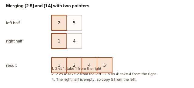 Two pointers walking two sorted halves, each step writing the smaller front value into the result
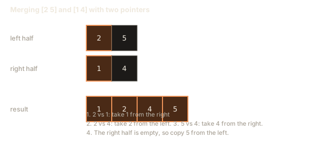
Why does this work? Because each section is sorted, the smallest remaining value in the whole merge must be at the front of one of the two sections. There is no other place it could be. The merge never has to look deeper, and it never has to go back.
The rule for ties matters too. When the two front values are equal, take the one from the left section. This keeps the order of equal values the same as in the input, which is what makes the sort stable. We come back to stability later in this lesson.
Merge sort in C++
A merge sort needs two functions. The first, mergeHalves, takes the two sorted sections and merges them. The second, mergeSort, does the splitting and calls mergeHalves on the way back up. The program below is complete. It reads a count and then that many numbers, sorts them, and prints them on one line.
Press Run and type this in the Input box:
7
38 27 43 3 9 82 10
The output is:
3 9 10 27 38 43 82Look closely at the merge function. It does not write into a while it is still reading from a. It writes into a temporary vector called tmp, and only at the end copies tmp back into the right place. Writing straight into a would overwrite values that have not been merged yet, and the result would be wrong. This is the reason the merge needs extra memory.
The mid value is computed with lo + (hi - lo) / 2, for the same overflow reason as in the previous lesson. The left section is lo to mid, and the right section is mid + 1 to hi. Those two sections never overlap, and together they cover the whole range.
The two loops after the main merge loop copy whatever is left over. One of the two sections is always exhausted first. The loops finish the other one. Forgetting these two lines is a common bug, and the common mistakes section shows what it looks like.
Trace a small example from start to finish
A small example makes the splitting visible. Sort 5 2 4 1. Split the array in the middle, so the halves are 5 2 and 4 1. Each half splits again, until every piece holds one value. Then merge up, from the bottom.
| Level | Pieces | What happens |
|---|---|---|
| Split 1 | 5 2 and 4 1 | The array is cut in the middle |
| Split 2 | 5, 2, 4, 1 | Each half is cut again, so every piece is one value |
| Merge 1 | 2 5 and 1 4 | Each pair of single values is merged |
| Merge 2 | 1 2 4 5 | The two sorted pairs are merged into the final array |
The final merge compares 2 with 1, then 2 with 4, then 5 with 4. That is three comparisons. The value 5 is left over and is copied at the end, with no comparison. Count all the comparisons in the example: one for 5 and 2, one for 4 and 1, and three for the final merge. That makes five in total.
The diagram below shows the same splits and merges as a tree. Read it from the top down to see the splits, and from the bottom up to see the merges.
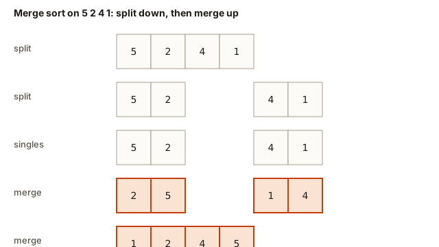 Merge sort on 5 2 4 1 split down to single values and merged back up into 1 2 4 5
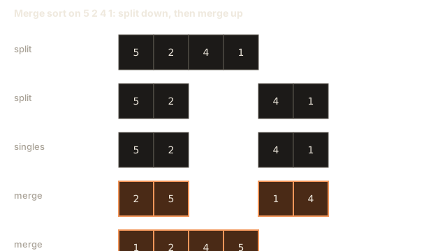
Now watch the same process on a longer array. The visualizer below sorts the values one merge at a time. Pay attention to the moment when a merge begins. The two sections are already sorted by the time the merge starts, because the recursive calls finish first.
Outlined bars are being compared. Filled bars were just swapped or written. Bars with a dark border are in their final place. Faded bars are outside the part being worked on.
Split the list in halves, sort each half, then merge the halves.
Why merge sort takes O(n log n)
There are two parts to the argument: how many levels of splitting there are, and how much work each level does.
First, the number of levels. Each split cuts the array in half, so a piece of size n becomes pieces of size n/2, then n/4, and so on, until the size is one. As in the previous lesson, that takes log n halvings. So there are about log n levels.
Second, the work per level. On any one level, the pieces are disjoint, so together they cover the whole array once. Merging all the pieces of one level touches each value once, which is n steps in total. The splitting itself costs only a single middle calculation per call, which is much less than n.
Multiply the two numbers. There are log n levels, each costing about n, so the total is n times log n. Computer scientists write this as O(n log n).
The important point is that this holds for every input. Merge sort does not get lucky on a sorted array, and it does not get unlucky on a reversed one. The shape of the splits does not depend on the values, so the cost does not depend on them either. That makes merge sort a dependable choice when the worst case matters.
The memory story is different. The temporary vector holds up to n values at a time, so the extra space is O(n). The recursion also uses a stack with about log n frames, which is smaller. Quick sort, the next lesson, uses less extra memory, but it does not promise the same time in the worst case.
Counting the work: an experiment
A formula is only useful if you can check it. The next program counts the comparisons that merge sort makes. It sorts reversed arrays of size 8, 16, 32, 64 and 128, and prints the count for each size. It takes no input.
The output is:
n=8 comparisons=12
n=16 comparisons=32
n=32 comparisons=80
n=64 comparisons=192
n=128 comparisons=448
Look at the pattern. For a reversed array of size n, the comparisons equal (n / 2) * log2(n). Check it: for 8 the formula gives 4 * 3 = 12, and for 128 it gives 64 * 7 = 448. The count grows a little faster than n, and it grows like n log n, exactly as the argument predicted.
Why does a reversed array give exactly half the merge size? Each merge takes the right section first, because every value on the right is smaller than every value on the left. The right section has n / 2 values, so there are n / 2 comparisons. The left values are copied at the end with no comparison. An already sorted array gives the same count, because then the left values come first and the comparisons come from the left section, which is also half the merge. You can check the sorted case with the practice exercises.
Notice that the counts are exact numbers, not estimates. When you analyse an algorithm in an interview, you can often predict the count exactly for a special input like this, and that is a strong way to show understanding.
Stability: keeping equal items in order
A sort is stable if items with equal keys stay in the same relative order after sorting. Suppose you have a list of people sorted by name, and you now sort them by age. People of the same age should still appear in alphabetical order by name. A stable sort gives you that for free. An unstable sort may mix them up.
The next program stores each person with a name and an age. It sorts by age only. Two people share age 25, and two share age 30. Read the output to see whether the original order is kept.
Press Run and type this in the Input box:
5
Ana 30
Ben 25
Cara 30
Dev 25
Esha 40
The output is:
Ben 25
Dev 25
Ana 30
Cara 30
Esha 40
Ben came before Dev in the input, and Ben still comes first after the sort. Ana came before Cara, and Ana still comes first. That is stability. The reason is the tie rule in the merge. When the two front ages are equal, the code takes the left item. The left section holds the items that appeared earlier in the input, because the split never reorders the items before the merge. So a tie always keeps the earlier item first.
Now change one character. Replace <= with < in the merge, so that the code takes the right item on a tie. Run the same input again. The output becomes:
Dev 25
Ben 25
Cara 30
Ana 30
Esha 40
Dev now comes before Ben, and Cara before Ana. Nothing else in the program changed, and the ages are still sorted correctly. The sort is wrong only in the order of equal items. This is why interviewers ask about stability, and why a single < versus <= is a real bug in production code.
Some languages and libraries offer both a stable sort and an unstable one, because the stable version is a little slower. Merge sort is the usual choice when you need stability and a guaranteed bound.
Merge two sorted lists
The merge step is useful on its own. Many problems give you two lists that are already sorted and ask for one list that combines them. Here is a function that does exactly that, followed by a program that reads two sorted lists from the input.
Type this in the Input box, and press Run:
4 3
1 4 7 9
2 3 8
The first line gives the size of each list. The output is:
1 2 3 4 7 8 9This version uses size_t, the unsigned type that vector::size() returns. Using size_t for indexes that are compared with size() avoids the sign warning shown earlier. The price is that you must be careful when you subtract from an unsigned number. This program never subtracts, so it is safe.
Choosing merge sort
The table compares merge sort with the other sorts you will see in this module and in the earlier lessons. It shows the cases that matter most for choosing one.
| Sort | Best case | Average case | Worst case | Extra memory | Stable |
|---|---|---|---|---|---|
| Merge sort | O(n log n) | O(n log n) | O(n log n) | O(n) | Yes |
| Quick sort (next lesson) | O(n log n) | O(n log n) | O(n squared) | O(log n) | No |
| Insertion sort | O(n) | O(n squared) | O(n squared) | O(1) | Yes |
| Bubble sort | O(n) | O(n squared) | O(n squared) | O(1) | Yes |
Pick merge sort when you need a guaranteed time bound, when stability matters, or when the data is a linked list, where splitting is cheap and no extra array is needed. Pick quick sort when memory is tight and the average speed matters more than the worst case. Insertion sort wins on tiny or nearly sorted arrays, because its constant factor is small.
Merge sort also handles data that does not fit in memory. You can sort chunks that fit, write them to disk, and merge the sorted chunks in one pass. Databases and large log processors do exactly this. The merge step is the part that makes the method work on data that is streamed instead of stored.
Common mistakes and what they look like
Using < instead of <= in the merge. This breaks stability, as the Ben and Dev example showed. The output is still sorted by the key, so the bug can hide until someone checks the order of equal items.
Forgetting to copy the leftovers. After the main loop, one section may still hold values. If you skip the two copy loops, the last values are missing from the result. The array then holds stale values at the end, and the output looks almost right. Always copy the rest of both sections.
Writing the result back to the wrong offset. The merged values belong at positions lo to hi, not at 0 to n - 1. Writing a[k] = tmp[k] instead of a[lo + k] = tmp[k] overwrites the start of the array when you merge a later section. The fix is to add lo.
Using a base case that is too narrow. Checking if (lo == hi) misses an empty range, which can happen when the array is empty. Use lo >= hi, which covers both.
Comparing an index with the size of a vector. This is the same warning as in the last lesson. If you compile with -Wall -Wextra, a loop such as for (int k = 0; k < tmp.size(); k++) prints this:
warning: comparison of integer expressions of different signedness: 'int' and 'std::vector<int>::size_type' {aka 'long unsigned int'} [-Wsign-compare]The warning is not an error, but it tells you the types disagree. Cast the size, as in (int)tmp.size(), which the programs in this lesson do.
Debugging a merge sort
When merge sort gives a wrong answer, the bug is almost always in the merge. The divide step is simple and the recursion is hard to get wrong. So debug the merge by itself. Write a tiny test with two sorted sections, call the merge, and print the result. Then try two edge cases: one section empty, and both sections holding equal values.
A quick check of the leftovers is also useful. Take the input 1 2 as the left section and 3 as the right section. The loop takes 1 and 2 from the left, then stops because i moves past mid. The right section still holds 3, so the copy loop for the right section must run. If that loop is missing, the output is missing the 3. The error is silent, and it only appears when the right section is longer or has values left over.
Remember that the sort returns the result in the same vector, so you can print the vector after each call to check the state. The visualizer above does exactly that for each merge.
The call order in detail
Follow the calls for 5 2 4 1 in your head. The first call to mergeSort covers the whole array. It calls mergeSort on 5 2, and that call calls mergeSort on 5, which returns at once. Then the call on 2 returns at once. Only after both of those finish does the 5 2 call run its merge, which writes 2 5 into the array. The caller then starts the second half, 4 1, and repeats the same steps. Finally the top level merges 2 5 with 1 4.
Every call waits for its children to finish before doing its own merge. This is the same stack behaviour as in the binary search lesson, where each frame waits for the frame it called. The stack depth is about log n, so the stack memory is small. The order is also what makes the merge safe, because the merge never reads a half that is still being sorted.
Edge cases you must test
Merge sort is simple, but its edge cases are easy to miss. Test each of these before you trust the code.
An empty array needs care. The program checks if (n > 0) before it calls mergeSort, because n - 1 would be -1 for an empty vector. The base case lo >= hi would also stop an empty range, but the explicit check makes the intent clear to the reader.
A single value is already sorted. The base case returns at once, and the merge is never called for it.
Two values in the wrong order give one merge with one comparison and one copy. Trace it on paper: 9 4 splits into 9 and 4. The merge compares 9 with 4, takes 4 first, and then copies 9.
All values equal gives a correct, stable result. With <= the merge always takes from the left, so the order never changes, and the output equals the input. The algorithm still does the full amount of work, because merge sort does not look for a sorted run. Some other sorts, such as insertion sort, do almost no work on sorted input.
An already sorted array also costs the full O(n log n) in the plain version. Interviewers sometimes ask whether you can do better. One fix is to check whether the largest value of the left half is at most the smallest value of the right half. If it is, the two halves are already in order, and the merge can be skipped. That check takes constant time, so sorted input then costs O(n), because the splits still happen but the merges do not. The worst case stays O(n log n).
Bottom-up merge sort
Merge sort can also be written without recursion. Start with runs of size 1, which are already sorted. Merge neighbouring pairs into runs of size 2. Then merge neighbouring pairs of those into runs of size 4, and keep doubling the run size on each pass, until one run covers the whole array. Each pass is one level of the split tree, read from the bottom up.
This version avoids deep recursion, and it is the natural form when the data arrives one block at a time. The total work is still O(n log n), and the extra memory is still O(n) for the merge buffer. In code, the same merge function works, with lo, mid and hi moving in steps that double each pass. Many libraries use a version of this idea, because the passes are simple to run in parallel.
Sorting data that does not fit in memory
Real systems sometimes need to sort more data than fits in memory. The method is called an external merge sort. Read the data in chunks that fit, sort each chunk in memory, and write each sorted chunk to a file. Then merge the sorted files. Read a few values from each file at a time, always take the smallest front value, and write it to the output file. The merge step is the same idea as before, extended to many inputs.
Log processors and database engines use this approach for large sorts. It works for the same reason as the in-memory merge: merging sorted inputs needs only the front value of each input. The program never needs all the data at once.
Interview questions on merge sort
Expect questions like these. Why is merge sort O(n log n) in every case? Why is it stable, and what would change the answer? How much extra memory does it need, and can you reduce it? How would you sort a linked list? How would you merge k sorted lists?
For the linked list question, a good answer splits the list with slow and fast pointers, sorts each part by recursion, and merges by relinking the nodes. That uses O(log n) stack space and no extra array. For k lists, merge pairs of lists in rounds. Each round touches every value once, and there are about log k rounds, so the total is O(N log k), where N is the total number of values.
A full trace on six values
Sort 9 3 7 1 8 2 and write down every merge. Each row shows the two halves and the result.
| Merge | Left half | Right half | Merged result |
|---|---|---|---|
Splits 9 3 | 9 | 3 | 3 9 |
Splits 9 3 7 | 3 9 | 7 | 3 7 9 |
Splits 1 8 | 1 | 8 | 1 8 |
Splits 1 8 2 | 1 8 | 2 | 1 2 8 |
| Top merge | 3 7 9 | 1 2 8 | 1 2 3 7 8 9 |
Read the table from top to bottom, because that is the order the merges finish. The left side builds 3 9, then 3 7 9. The right side builds 1 8, then 1 2 8. The top merge compares 3 with 1 and takes 1, compares 3 with 2 and takes 2, compares 3 with 8 and takes 3, compares 7 with 8 and takes 7, and compares 9 with 8 and takes 8. The 9 is left over and is copied at the end. That is five comparisons in the top merge, and the final output is 1 2 3 7 8 9.
There are five merges in total, one for each internal node of the call tree, and six single-value leaves. So the recursion makes 11 calls in all. The number of merges is always one less than the number of values, which is a useful check when you trace a larger example.
Moves versus comparisons
A comparison looks at two values. A move copies a value from one place to another. In each merge, every value is copied into the temporary vector and then copied back, so each value gets two moves per level. Over all the levels that is about 2 n log n moves, while the comparisons are at most n log n. The two counts differ by a constant factor, but both grow in the same way.
In practice, the time of a large sort is often limited by how much data moves through memory, not by how many comparisons happen. That is one reason merge sort on very large arrays is limited by memory speed, and why libraries pay attention to the layout of their temporary storage.
Why the bound holds for every input
The split always produces halves of size n / 2, rounded one way or the other, no matter what the values are. So the shape of the call tree depends only on n. Every level of that tree has merges that together cover the whole array. The bound therefore holds for every input, without a lucky choice and without a special case.
This is the main difference from quick sort. In quick sort, the shape of the tree depends on the values, because the pivot decides where the split falls. A good pivot gives a balanced tree, and a bad pivot gives a long, thin one.
Library sorts built on merging
Several widely used sorts are built on merging. Python's built-in sorted uses Timsort, which finds runs of values that are already in order and merges them. Java's sort for objects uses a merge-based algorithm too. C++'s std::stable_sort typically uses a merge strategy. Libraries add tricks, such as insertion sort for short runs and detection of existing order, but the merge is the core. Knowing this lesson lets you read those libraries' documentation and understand why they are stable.
The merge as a small state machine
It helps to think of the merge as a machine with three values in its state: the left index i, the right index j, and the output position. At each step the machine looks at the two values under i and j. It moves one value to the output and advances the index of the side it took from. The machine stops moving values when either side is empty. Then it copies whatever is left on the other side.
Each step does exactly one of two things: take from the left, or take from the right. Each value is taken exactly once, so the merge makes exactly n takes for n values, plus the comparisons that decide each take. This view also shows why the code is safe. The machine never looks past the end of either side, because the loops check i <= mid and j <= hi before every comparison.
The same view explains the tie rule. When both values are equal, the machine picks the left side. The output then keeps the left value first, which is the same order it had in the input. A machine that picked the right side on ties would reorder equal values, and the sort would no longer be stable.
Sorted input: what merge sort really does
Consider a sorted array of 8 values. Every merge finds that all left values are smaller than all right values. So the machine takes every left value in turn, comparing each one with the front of the right side, and then copies the right side at the end. The comparisons happen only while the left side has values. A merge of size 8 with two sides of size 4 makes 4 comparisons. The whole sort makes 12 comparisons, the same count as the reversed array of size 8 from the counting program.
This surprises many students. They expect a sorted input to be cheap, but plain merge sort still splits and merges everything. For this array it makes the same 12 comparisons as the reversed array. Only the version with the extra check, which skips a merge when the halves are already in order, does less work on sorted input.
Practice
Work on paper first, then check your code with a program.
- Sort the array
4 1 3 2by hand using merge sort. Draw the split tree, and write the sorted pieces at each merge.
Solution
Split into 4 1 and 3 2. Split again into 4, 1, 3, 2. Merge 4 with 1 to get 1 4. Merge 3 with 2 to get 2 3. Merge 1 4 with 2 3 to get 1 2 3 4. Three merges happen in total, and each value is copied once per level.
- Change the merge so the array is sorted in descending order, and keep the sort stable. Hint: only one comparison changes.
Solution
Take the left value when it is greater than or equal to the right value. The condition a[i] >= a[j] keeps equal items in their original order and sorts from largest to smallest.
- Write
mergeHalvesfor two sorted sections that you can call with anylo,midandhi. Test it with the sections2 5and1 4, and check that it prints1 2 4 5.
Solution
The function from this lesson already works with any lo, mid and hi. Put 2 5 1 4 in an array, call mergeHalves(a, 0, 1, 3), and print the array. The output is 1 2 4 5.
- Sort a
vector<string>by length, and keep strings of the same length in their original order. Hint: the comparison usessize().
Solution
Compare s[i].size() <= s[j].size() in the merge, and keep the rest of the code the same. The <= keeps ties in the left-first order, which keeps equal lengths stable.
- Merge sort on an already sorted array of 8 values makes how many comparisons? Predict the answer, then check it with the counting program after changing the input line to
a[i] = i + 1;.
Solution
For a sorted array, the left section is always smaller, so the merge takes all left values with a comparison each, and then copies the right values. Each merge costs the size of its left section. For 8 values there are four merges of size 2 (cost 1 each), two merges of size 4 (cost 2 each), and one merge of size 8 (cost 4). That is 4 + 4 + 4 = 12. The program prints n=8 comparisons=12.
- Given
ksorted lists, merge them into one sorted list by using merge sort's pattern: merge pairs of lists, then merge the results, until one list is left. What is the total cost in terms ofN, the total number of values, andk?
Solution
Merging the lists in pairs is a divide and conquer pattern. There are about log k rounds. In each round, every value is copied once, so each round costs about N. The total cost is O(N log k). Merging all the lists one after another costs more, because the list grows and is copied again and again.
- Sort a singly linked list with merge sort. Explain how to find the middle, and what changes in the merge step. Do not write a full program.
Solution
Use two pointers, a slow one that moves one node per step and a fast one that moves two. When the fast pointer reaches the end, the slow pointer is at the middle. Cut the list after the middle to get two lists. Sort each one by recursion, and merge the two sorted lists by relinking nodes instead of copying values. The merge needs no extra array, so the extra memory is O(log n) for the recursion stack.
- Explain in your own words why merge sort is stable and quick sort, as usually written, is not.
Solution
Merge sort takes the left item on a tie, and the left item was earlier in the input, so equal items keep their order. Quick sort swaps items across the array during partition. A swap can move an equal item past another equal item that was originally in front of it, so their order changes.
What you now know
- Merge sort splits the array, sorts each half by recursion, and merges the two sorted halves.
- The merge uses two indexes and a temporary vector. It always writes the smaller front value.
- The number of levels is log n and each level costs n, so the time is O(n log n) for every input.
- The extra memory is O(n) for the temporary storage.
- Taking the left item on a tie keeps equal items in order, so the sort is stable.
- Counting comparisons on special inputs gives exact numbers that check your analysis.
- The merge step alone solves the problem of combining two sorted lists.