Why this matters
Time is only half of the cost of a program. The other half is memory. A program that is fast but needs 40 gigabytes will crash on a laptop. A phone app that keeps a copy of every photo in memory will be killed by the operating system. A server that gives each request an extra megabyte runs out of room when a thousand requests arrive together.
Space complexity is the same idea as time complexity applied to memory: how does the amount of memory grow as the input grows? This lesson teaches how to count it, including the memory that recursion uses without you noticing. It also teaches the trade between time and space, which is the most common way to speed a program up, and a third notion, amortised cost, which explains why appending to a growing list is cheap even though sometimes it is expensive.
What counts as space
When we say a function has space complexity O(n), we mean that the memory it uses grows in proportion to n. But memory used by what? Two different quantities are in play.
- Input space is the memory that holds the input itself, such as the list you were given. You did not create it, and you cannot avoid it.
- Auxiliary space is the extra memory your function allocates while it runs: new lists, dictionaries, counters and the stack of function calls.
By convention, "space complexity" in interviews means auxiliary space, unless the problem says otherwise. If a function takes a list of n numbers and uses a handful of variables, it uses O(1) extra space, although the input itself takes O(n).
An everyday picture: you are asked to sort a pile of exam papers on a desk. Doing it by swapping papers within the pile needs no extra table: O(1) extra space. Doing it by laying all the papers out on a second table in sorted order needs a second table as big as the first: O(n) extra space. Both give a sorted pile. They differ in how much room they need.
Memory cost is counted the same way as time: we ignore constants. A variable that holds one number is one unit. A list of n numbers is n units. A grid of n rows and n columns is n * n units.
O(1) space: a few variables
A function whose extra memory does not grow with the input has constant space.
17
6
Both functions use a few variables (best, x, count, ch) no matter how long the input is. The loop reads one element at a time. That is O(1) auxiliary space. Doubling the length of the list does not add a single variable.
O(n) space: a copy or a table that grows with the input
Whenever a function builds a new collection with one entry per input item, it uses O(n) space.
[1, 4, 9, 16, 25]
[1, 3, 6, 10, 15]
Each function creates a new list with n entries, so each uses O(n) extra space. Time is O(n) as well. The result list counts as auxiliary space because we created it, even though we hand it back to the caller. (Some people do not count the output when they compare algorithms. Say which convention you use if it matters.)
Space can also grow without a visible append. Slicing copies, sorted() returns a new list, list(items) copies, and a list comprehension builds a list. Each costs space proportional to the number of items copied.
In place: reusing the input
An algorithm is in place when it changes the input directly and needs only O(1) extra space. Reversing a list is the classic case. Compare two versions.
[6, 5, 4, 3, 2, 1]
[1, 2, 3, 4, 5, 6]
[6, 5, 4, 3, 2, 1]
Both take O(n) time. The first leaves data untouched and builds a second list, O(n) space. The second swaps pairs from the two ends and uses just two index variables, O(1) space. The price of in-place work is that the original is gone. If the caller needs the old order, the in-place version is the wrong choice. This kind of trade-off, safety against memory, is a decision you make with your eyes open.
O(n^2) space: tables
A two-dimensional table with n rows and n columns has n * n cells. Programs that fill tables, such as the dynamic programming methods later in the course, use O(n^2) space.
[1, 2, 3, 4]
[2, 4, 6, 8]
[3, 6, 9, 12]
[4, 8, 12, 16]
10 100 cells
100 10000 cells
1000 1000000 cells
At n = 1,000 the table has a million cells. In Python each cell is a pointer of 8 bytes, plus the integer objects it points to, so a table of a million cells takes tens of megabytes. At n = 100,000 the table would need ten billion cells, far more memory than most computers have. Quadratic space becomes a wall faster than quadratic time does, because memory is a hard limit: when you run out, the program crashes instead of slowing down.
MemoryErrorPython raises MemoryError when it cannot get enough memory for an object, for example when you try to build a list with hundreds of billions of elements. Other systems may kill the process without a message, or the machine may slow to a crawl as it swaps memory to disk. The fix is to find an algorithm with smaller space, or to process the data in pieces.
The hidden cost: the recursion stack
Recursion uses memory even when you never create a list. Each call that has not yet returned occupies a stack frame: a block of memory holding the arguments, local variables and the place to return to. The frames stack on top of each other, which is why this region of memory is called the call stack.
Think of a pile of sticky notes on your desk. Every time you are interrupted to do a sub-task, you write down where you were on a note and put it on the pile. You finish the sub-task, then take the top note off and continue. The height of the pile is the number of interruptions waiting at once.
Here is the call stack for a recursive factorial at its deepest point.
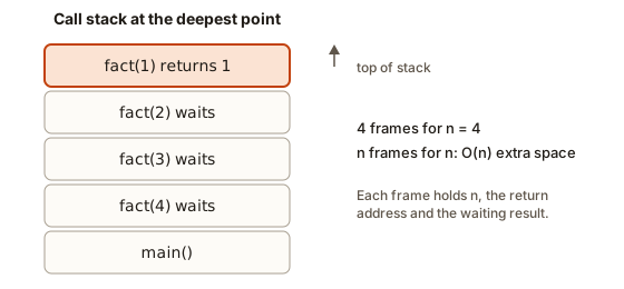 Call stack of four frames for factorial of 4, with the newest call on top
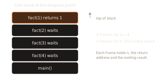
The rule for recursion space: the extra space is the maximum depth of the call stack, times the size of one frame. If each frame has constant size, it is just the maximum depth.
1 1
5 5
10 10
50 50
The second column is how many calls were open at once at the deepest point. Factorial of 50 keeps 50 frames. The depth is n, so the recursive factorial uses O(n) auxiliary space, while the loop version uses O(1). Both take O(n) time.
Use the stack visualizer to see frames pushed and popped.
removed: nothing
The top is the box marked top. An outlined box was just pushed or peeked.
The stack is empty. The last item pushed is the first one popped.
Push and pop on the stack, and picture each push as a function call starting and each pop as a call returning. Watch how the stack grows only when you push faster than you pop; the highest point reached is the memory you needed.
The next table compares the stack depth of the recursive algorithms from the last lesson.
| Function | Time | Max stack depth | Extra space |
|---|---|---|---|
factorial, fact(n - 1) | O(n) | n | O(n) |
| binary search, recursive | O(log n) | log n | O(log n) |
| merge sort | O(n log n) | log n | O(n) for merged lists (the stack itself is O(log n)) |
| naive Fibonacci | about O(1.6^n) | n | O(n) |
| Tower of Hanoi | O(2^n) | n | O(n) |
Two rows deserve a closer look. Naive Fibonacci has more than a billion calls for n = 40, but they are not all alive at once. The first call goes down the left branch to depth n, returns, then goes down the next branch. At any moment the open calls form a single path from the root to the current call. So the space is O(n), the longest path, while the time is exponential. The number of calls and the number of simultaneous calls are different measures.
Merge sort's stack is only log n deep, but the merging step builds new lists, and the merged lists at one level add up to n items. So its auxiliary space is O(n).
The question "does this recursion fit in the stack" matters in practice. Languages have a limit on depth. Python's default is about 1,000 frames.
True
500
RecursionError: maximum recursion depth exceeded
A depth of 500 is fine. A depth of 100,000 raises RecursionError. The remedy is to write the loop version, which uses O(1) space, or to restructure the recursion so it is shallower, for example by halving instead of stepping by one. Java reports the same situation as java.lang.StackOverflowError, and C++ simply crashes with a segmentation fault, because the stack is a fixed-size region of memory, typically 1 to 8 megabytes.
Time against space: trading one for the other
Many speedups work by spending memory. You store something you computed so you do not compute it again. Three examples show the trade.
Example 1: the duplicate check. Two ways to detect a duplicate in a list of n items.
True True True| Method | Time | Extra space |
|---|---|---|
| compare every pair | O(n^2) | O(1) |
| sort, then check neighbours | O(n log n) | O(n) for the sorted copy (O(1) if you sort in place) |
| set of seen values | O(n) | O(n) |
There is no free lunch in this table. The quadratic method uses the least memory but the most time. The set method uses the most memory but the least time. The sorting method sits between. Which is right depends on the numbers. For n = 100 the quadratic one is fine. For n = 10 million the set may be too big for the machine, while sorting in place might fit.
Example 2: memoisation. Remember computed results in a table so each subproblem is solved once. Naive Fibonacci uses exponential time and O(n) stack space. With a stored table of size n it uses O(n) time and O(n) space.
832040 832040
2880067194370816120 2880067194370816120
The iterative version keeps only the last two values: O(n) time and O(1) space. Same answers, and each step down from the exponential version came from understanding what the program really needs to remember. This pattern, keeping only the part of a table you still need, is a favourite interview optimisation for dynamic programming.
Example 3: prefix sums. Suppose you must answer many questions of the form "what is the sum of items from position a to position b?". Summing each time costs O(n) per question. Precompute a table of running totals once, O(n) time and O(n) space, and every question costs O(1).
[0, 4, 5, 12, 15, 24, 26]
26
19
3
The table prefix holds the total of the first k items at position k, so the sum from a to b is the difference of two entries. If you ask a thousand questions about a list of a hundred thousand items, the table saves about 10^8 steps in exchange for 100,000 extra cells.
Remember the pattern: precomputation costs space and one-time work, then makes later work cheap. It is what an index in a database does, what a cache does, and what a lookup table in a game does.
Amortised cost: cheap on average, expensive sometimes
The last idea in this lesson explains something you have used already. When you call append on a Python list, the list sometimes has no free slot at the end. The computer then allocates a bigger block of memory, copies every item over and discards the old block. That copy costs O(n). Yet we say append is O(1). How can both be true?
The answer is amortised analysis: instead of the cost of one operation, we study the total cost of a sequence of operations and divide by the number of operations. If a rare operation is expensive but pays for many cheap ones, the average per operation stays small. This is not the same as the average case, which averages over random inputs. Amortised cost is a guarantee about any sequence of operations, with no randomness assumed.
An everyday picture: you drive a car and fill the tank once a month. That one stop takes 10 minutes, while all other days cost zero minutes. Averaged over 30 days it is 20 seconds a day. The long stop is rare and the average is small.
How a dynamic array grows
A dynamic array, which is what a Python list or a Java ArrayList or a C++ vector is, is a block of memory with a capacity (how many slots it has) and a size (how many slots are in use). While size is below capacity, an append writes into the next free slot: one step. When the array is full, it allocates a block twice as large, copies all items over, then appends.
Here is a simulation that counts the cost of each append, one unit for the write and one unit for each item copied during growth.
append  1: cost  1, capacity now 1
append  2: cost  2, capacity now 2
append  3: cost  3, capacity now 4
append  4: cost  1, capacity now 4
append  5: cost  5, capacity now 8
append  6: cost  1, capacity now 8
append  7: cost  1, capacity now 8
append  8: cost  1, capacity now 8
append  9: cost  9, capacity now 16
append 10: cost  1, capacity now 16
append 11: cost  1, capacity now 16
append 12: cost  1, capacity now 16
append 13: cost  1, capacity now 16
append 14: cost  1, capacity now 16
append 15: cost  1, capacity now 16
append 16: cost  1, capacity now 16
append 17: cost 17, capacity now 32
total cost: 48  per append: 2.82
Look at the cost column. Most appends cost 1. The expensive ones come at i = 2, 3, 5, 9 and 17, which are one more than a power of two, and each costs i, because it copies all items. The picture shows the same story.
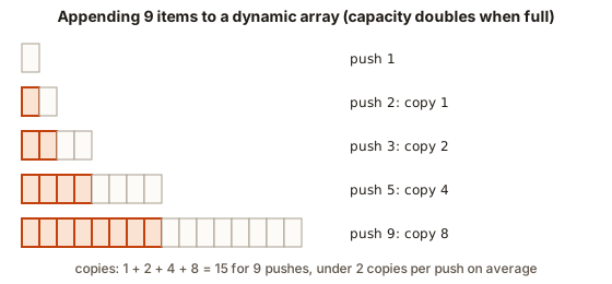 Capacity rows 1, 2, 4, 8 and 16 with the copied cells shaded
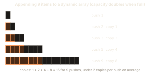
The total for 17 appends is far less than 17 * 17. To see the pattern for larger n, compute the total cost and divide by n.
10 25 2.5
100 227 2.27
1000 2023 2.023
100000 231071 2.311
1000000 2048575 2.049
The last column, cost per append, stays under 3 however large n gets. It never grows. That is the meaning of O(1) amortised.
Why it works: the sums
Here is the argument in math. When we grow from capacity k to 2k, we copy k items. The growth happens at sizes 1, 2, 4, 8, ..., up to the last power of two below n. The total copying is
1 + 2 + 4 + 8 + ... + 2^m, where 2^m < n.
This geometric series sums to 2^(m+1) - 1, which is less than 2n. So the copying over all n appends is under 2n, and the writes cost n. The total is under 3n, which gives under 3 per append. That matches the table above. The key fact: the last doubling costs about half of everything.
The banker's view
There is a second way to see it, the accounting method. Charge every append a fixed price of 3 coins. One coin pays for writing the new item. Two coins go into a savings account attached to that item. When the array doubles, the items that were added since the last doubling carry enough savings to pay for copying all items. Half of the items in a full array each brought 2 coins since the last growth, which is enough to copy the whole array (the older half pays with its 2 coins as well). Since the coins never run out, the real cost of any sequence of appends is at most 3 coins times the number of appends. So the amortised cost is 3: O(1).
Growth must multiply
What if the array grew by a fixed amount, say 10 slots at a time, instead of doubling? Then there would be a copy every 10 appends, each copying everything so far.
1000 50600 50.6
10000 5006000 500.6
100000 500060000 5000.6
The cost per append grows with n: about n / 20 per append, so the total is quadratic. Adding a constant is not good enough. The array must grow by a constant factor, doubling or multiplying by 1.5, for the amortised cost to stay constant. Real implementations use factors between about 1.125 and 2. Python's list over-allocates by roughly an eighth of its size plus a small constant, which is still a constant factor and so still gives O(1) amortised. The exact numbers are an implementation detail that changes between versions, but the principle does not.
The trade is space. After doubling, up to half of the array is empty. So a dynamic array uses between n and 2n slots: O(n) space, with some waste.
Other amortised examples
Queue from two stacks. A queue gives items in the order they arrived. You can build one from two stacks: push onto an "in" stack, and when you need to pop and the "out" stack is empty, move everything from "in" to "out", which reverses the order. One pop may move n items: O(n). But each item moves at most once, from in to out, so over m operations the total movement is at most m. Amortised cost per operation: O(1).
1 2 moves so far: 5
3 4 5 6 moves in total: 6
The first pop moved 5 items. The next four pops moved nothing, because the outbox already had items in the right order. The sixth item moved once more. The total movement, 6 moves for 6 items, is one move per item: amortised O(1).
Hash table resizing. A hash table, which you will build later in this course, also doubles when it gets too full and re-inserts every key. The same sum shows that inserts are O(1) amortised.
String building. In Python, text += piece in a loop can look quadratic, since each concatenation could copy the text. In practice CPython has an optimisation that often avoids the copy, but you cannot rely on it across versions or other implementations. The portable method is to collect pieces in a list and join them once at the end, which is O(n) in total.
0-1-2-3-4Reading space off code: a checklist
Space analysis follows the same habit as time analysis. Walk through a function and list every place where memory is allocated.
- Name the input sizes, exactly as for time.
- List every new container: each list, dictionary, set, string and table you create. Write down its largest possible size in terms of n.
- Check the library calls:
sorted,list, slices,join,copy, comprehensions,split. Each makes a new object. - Check the recursion: find the deepest chain of open calls, and multiply by the space each frame needs.
- Take the largest, not the sum of all: if two containers exist at the same time, add them; if one is freed before the next is built, only the largest counts. Then drop constants, as always.
Apply it to a function that finds the words two sentences have in common.
['on', 'sat', 'the']Let p be the number of words in the first sentence and q the number in the second. The two sets use O(p) and O(q). The call a.split() builds a temporary list of p words, and sorted(words_a) another list of up to p words. Not all of them are alive at the same moment, but a few are, and constants vanish anyway. The auxiliary space is O(p + q). The result list is at most min(p, q) long, which is already covered. Time is O(p log p + q): the sort dominates for the first sentence and building the second set is linear.
Notice the thing a careless count misses. A reader who looks only for lists named result or table sees one list, shared, and answers "O(min(p, q))". The sets and the split lists are the real cost.
Space of familiar algorithms
You now have the tools to state the space cost of the algorithms from earlier modules. Keep this table as a reference. It uses the standard textbook versions.
| Algorithm | Time (worst) | Auxiliary space |
|---|---|---|
| linear search | O(n) | O(1) |
| binary search, loop | O(log n) | O(1) |
| binary search, recursive | O(log n) | O(log n) |
| bubble, selection, insertion sort | O(n^2) | O(1) |
| merge sort | O(n log n) | O(n) |
| quicksort | O(n^2), usually O(n log n) | O(log n) typical stack, O(n) worst |
| heap sort | O(n log n) | O(1) |
| counting a frequency table | O(n) | O(k) for k distinct keys |
| building all subsets | O(n * 2^n) | O(n * 2^n) if stored, O(n) if generated one at a time |
The last row shows another lever: you can sometimes avoid storing everything by producing answers one at a time and handling each as it appears. In Python this is what a generator does. A generator is a function that hands out values one by one with yield and remembers where it stopped.
65536 16All 65,536 subsets of 16 items were visited, but only one subset was alive at a time, so the space stays small, O(n), against O(n * 2^n) if we had stored them all in a list. Time is the same. The cost of the generator is that you can walk through the answers only once, in order.
What happens inside: memory, the stack and the heap
Where does all this memory live? A running program has two main areas.
The stack holds the frames of function calls. It is fast, because allocating a frame just moves a pointer, and it is small, with a fixed limit. When a function returns, its frame is released automatically.
The heap holds objects that outlive a single call, such as the contents of a list, a dictionary or a string. It is large, limited by the machine's memory, and slower to manage. In Python, a variable holding a list stores only a reference, a small address, on the stack, while the list's items are on the heap.
This split explains what we measured. The recursion depth consumes stack space. The lists and tables we build consume heap space. RecursionError comes from the first limit, MemoryError from the second.
A dynamic array's growth happens on the heap. The runtime asks for a new, larger block, copies the old contents and releases the old block. For a short moment both blocks exist, so growing needs about 1.5 to 3 times the memory of the data. That is why a program can run out of memory in the middle of a big append loop.
Memory also has a time cost. Reading items that sit next to each other in an array is fast, because the processor loads a whole line of neighbouring bytes at once into its cache. Following scattered pointers is slower. This is part of why a plain array often outperforms a structure with better Big-O at moderate sizes.
Common mistakes
Mistake 1: forgetting the recursion stack. "This uses no extra memory, only a function" is wrong when the function recurses. A recursion of depth n uses O(n) space. State it: "O(n) from the call stack."
Mistake 2: counting the input as extra space. If the input is a list of n items and the function only uses a few variables, the auxiliary space is O(1). Do not say O(n) just because the input has n items.
Mistake 3: forgetting hidden copies. items[1:], sorted(items), list(items), "".join(...) and str + str create new objects. A recursion that slices its input at each of n levels allocates n + (n-1) + ... + 1 items in total, although not all are alive at the same time.
Mistake 4: confusing amortised with average. Amortised is a worst-case guarantee over a sequence, with no randomness. Average case depends on a probability model of the inputs. A single append can still cost O(n); the guarantee is that n appends never cost more than O(n) in total.
Mistake 5: believing in-place always means O(1). Some in-place algorithms use a recursion stack. Quicksort sorts in place without a second array but uses O(log n) stack space on average, and O(n) in the worst case. "In place" means no big auxiliary array, not necessarily zero extra memory.
Mistake 6: growing by a constant. A custom dynamic array that grows by a fixed number of slots has O(n) amortised appends. Grow by a factor.
Real error messages for this lesson.
RecursionError: maximum recursion depth exceededToo many open calls, as we saw above. Check for a missing base case; if the base case is right, convert to a loop.
MemoryErrorThe program asked for more heap memory than is available. In a Linux process you may instead see the message Killed, which comes from the operating system when it stops a program that uses too much memory. Look for a table, list or copy that grows with n or n^2.
java.lang.StackOverflowError
java.lang.OutOfMemoryError: Java heap space
These are the Java names for the same two failures, the first from the stack and the second from the heap.
A debugging walkthrough: the job that dies at one million rows
A teammate writes a script to find the pairs of products bought together. It works on 2,000 orders and is killed at 200,000.
('bread', 'jam') 1
('bread', 'milk') 1
('bread', 'tea') 1
('jam', 'tea') 1
('milk', 'tea') 2
Step 1: say what n is. Let o be the number of orders and k the largest basket size. Step 2: time. Three nested loops, but two of them run over a basket: o * k^2 pair steps, small if baskets are small. Step 3: space. The counts dictionary has one entry per distinct pair. If there are p distinct products, the number of distinct pairs can reach p * (p - 1) / 2: with 50,000 products, over a billion pairs. That is the space bomb. The dictionary grows with the number of distinct pairs that appear, and a large catalogue produces too many.
Step 4: what can be done? Options, each with a cost. Keep only pairs that appear at least some number of times (needs more passes). Process the orders in batches and write partial counts to disk. Count only pairs that include a product of interest. Approximate with a counting sketch, a structure that trades exactness for fixed size. The right choice depends on what the report must show. The skill being exercised here is to ask where memory grows, in terms of the data, before the program is run at scale, instead of finding out from a crash.
Where this shows up in real life and interviews
Interviews. Every solution should end with "time O(...) and space O(...)". Typical follow-ups are "can you do it in O(1) space?" (usually by working in place, or with two pointers, or by reusing the input) and "what is the space of the recursion?" (the depth). Learning to say "O(log n) stack space, O(n) for the merge buffer" is a strong signal.
Systems. Caches trade memory for speed, and choosing what to keep is the whole design problem. Mobile apps have small memory budgets, so they choose in-place or streaming algorithms. Big-data tools process files in chunks because the file is larger than memory.
Language design. Dynamic arrays are everywhere because the amortised O(1) append makes them a good default. Knowing why helps you trust append in a loop and distrust insert(0, x).
Practice
1. (Easy) State the auxiliary space of each.
def a(items):
    total = 0
    for x in items:
        total += x
    return total

def b(items):
    return [x * 2 for x in items]

def c(n):
    return [[0] * n for _ in range(n)]
Solution
a uses O(1): one variable. b uses O(n): a new list with n entries. c uses O(n^2): n rows each of n zeros.
2. (Easy) What is the stack depth of def f(n): return 0 if n == 0 else 1 + f(n - 1) for n = 6? What is its space?
Solution
The calls f(6), f(5), ..., f(0) are all open at the deepest point: 7 frames. In general n + 1 frames, so O(n) space.
3. (Easy) An empty dynamic array has capacity 1 and doubles when full. How many items does it copy during growth while you append 8 items, and what is the capacity at the end?
Solution
Growth happens when appending the 2nd item (copy 1), the 3rd (copy 2) and the 5th (copy 4). The total copied is 1 + 2 + 4 = 7. The capacity after 8 items is 8; the ninth item would trigger a copy of 8.
4. (Medium) Write the in-place version of "move all zeros to the end, keeping the order of the other items" and give its time and space.
Solution
Keep a write position and copy each non-zero item to it, then fill the rest with zeros.
[1, 3, 12, 5, 0, 0, 0]Two passes, so O(n) time. Only the indices write and read are extra, so O(1) space.
5. (Medium) What is the space complexity of this recursive function, counting the stack? What is its time?
def half_sum(n):
    if n <= 0:
        return 0
    return n + half_sum(n // 2)
Solution
n halves each call, so the depth is about log2(n) + 1. Each frame is constant size. Space O(log n). The time is also O(log n), because there is one call per level and constant work in each.
6. (Medium) Merge sort allocates a list in each merge. Explain why its auxiliary space is O(n) and not O(n log n), even though it does log n levels of merging.
Solution
Merged lists are created and then discarded as the recursion unwinds. At any moment, the lists that are alive belong to calls on the current path from the root to a leaf, with sizes n, n/2, n/4, ..., summing to at most 2n. The lists from earlier levels have already been released. So the peak is O(n). Allocating n items at each of log n levels adds up to O(n log n) total allocation over time, but not O(n log n) at once.
7. (Medium) Fill the blanks: appending n items to a dynamic array that doubles costs under ___ copies in total, so each append costs ___ amortised.
Solution
Under 2n copies in total, so each append costs O(1) amortised: under 3 units counting the write. The reason is the geometric series 1 + 2 + 4 + ... + 2^m < 2n.
8. (Medium) A function builds a list by calling result = [x] + result for each of n items (insert at the front). Is this O(n)? What is the cost, and how do you fix it?
Solution
Each [x] + result builds a new list holding all previous items plus one, which costs about the current length. The total is 1 + 2 + ... + n = n(n+1)/2: O(n^2) time. Append instead and reverse once at the end: result.append(x) for all items, then result.reverse(). That is O(n) total.
9. (Hard) A grid of 5,000 by 5,000 integers must be processed to find, for each cell, the sum of all cells above and to its left. Compute the cost of a full table and describe a way to use less space.
Solution
The full table has 25,000,000 cells; at 8 bytes per pointer in Python that is 200 MB for pointers, plus integer objects, so it is heavy. Each cell of the new table needs only the cell to its left and the row above, so you can keep just the previous row, 5,000 cells. If the answers must be output in order, write each finished row and discard the older one. Space drops from O(n^2) to O(n), while time stays O(n^2). This is the same trick as the Fibonacci with two variables.
10. (Hard) Show that growing by a constant c slots makes n appends cost n^2 / (2c) copies, by summing the copy sizes.
Solution
Copies happen at sizes c, 2c, 3c, ..., n (roughly), each copying that many items. There are n / c copies. The sum is c * (1 + 2 + ... + n/c) = c * (n/c)(n/c + 1) / 2, about n^2 / (2c). So the cost is quadratic in n for any fixed c. Check with the earlier program: for n = 100,000 and c = 10, the expected number of copies is about 500 million.
What you now know
- Space complexity counts the extra memory a function allocates as the input grows; the input itself is not counted as auxiliary space.
- Variables give O(1), a copy or table with one entry per item gives O(n), and a grid gives O(n^2).
- Recursion uses stack memory equal to its maximum depth: factorial uses O(n), binary search O(log n), and a naive Fibonacci uses O(n) space despite making exponentially many calls.
- Time and space trade off: sets, memoisation and prefix sums spend memory to save time, and in-place algorithms spend time or safety to save memory.
- Amortised cost averages a sequence of operations: doubling a dynamic array copies under
2nitems for n appends, so append is O(1) amortised, as long as capacity grows by a factor and not by a constant.