Why this matters
In the last lesson you learned to boil a step count down to its dominant term. That leaves a short list of answers that keep coming back. A handful of growth rates cover nearly every program you will write: constant, logarithmic, linear, linearithmic, quadratic, cubic, exponential and factorial. Each has a recognisable code shape and a real-world feel.
If you know the list, you can do two valuable things. You can look at a loop and name its class in seconds. And you can work backwards from a problem: "n is up to 100,000 and I have one second, so I need something near O(n log n)". That second skill decides whether a solution passes a coding contest, survives an interview, or holds up in production.
The ladder of growth rates
Think of the classes as rungs on a ladder, ordered from slowest-growing at the bottom to fastest-growing at the top.
| Class | Name | Typical shape of code | Example |
|---|---|---|---|
O(1) | constant | a few statements, no loop over the input | read items[5] |
O(log n) | logarithmic | the problem halves each step | binary search |
O(n) | linear | one loop over the input | find the maximum |
O(n log n) | linearithmic | halve repeatedly, do n work per level | merge sort |
O(n^2) | quadratic | loop inside a loop | compare every pair |
O(n^3) | cubic | three nested loops | naive matrix multiply |
O(2^n) | exponential | try every subset | list all subsets |
O(n!) | factorial | try every ordering | list all permutations |
Anything lower on the ladder is faster for large n. We will take each rung in turn, show a program that lives there, and trace it.
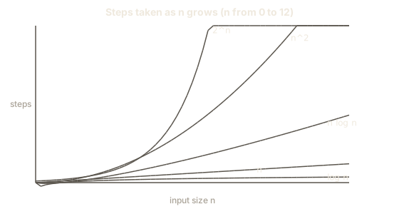
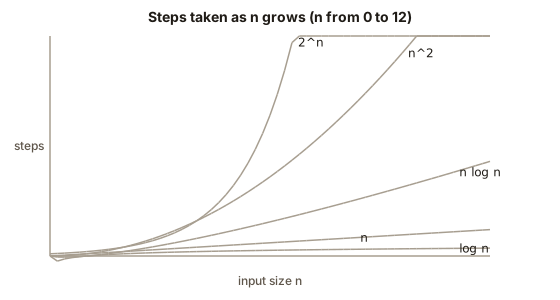 Steps against n for log n, n, n log n, n squared and 2 to the n
O(1): constant time
A constant-time operation takes the same number of steps whatever the input size. The everyday picture is a light switch: flipping it takes the same effort whether the house has two rooms or two hundred.
30
50
18
5
[10, 20, 30, 40, 50, 60]
Why is items[2] constant? A list stores its elements next to each other in memory. To reach position 2 the computer takes the address where the list starts and adds 2 times the size of one slot. That is one multiplication and one addition, whether the list holds five items or five million. This is why arrays are the backbone of so many structures: any position is reachable in one jump.
len(items) is constant because Python stores the length alongside the list. prices["coffee"] is constant on average because a dictionary turns the key into a position by arithmetic (a hash function) and jumps there. append is constant on average too, with a subtlety we resolve in lesson four.
Constant time does not mean fast. It means the time does not depend on n. A function that always does a million steps is O(1), although you would not want to call it in a loop.
O(log n): logarithmic time
A logarithm answers the question "how many times can I halve n before I reach 1?". Written log2(n), it is the exponent you need: 2^5 = 32, so log2(32) = 5. For quick intuition, log2 of a thousand is about 10, of a million is about 20, and of a billion is about 30.
That last number is the magic of this rung. A billion items, and you do about thirty steps. Logarithmic algorithms feel instant at any size.
The everyday picture is guessing a number from 1 to 100 when a friend says only "higher" or "lower". Guess 50. If higher, the answer is in 51 to 100: half the possibilities gone with one question. Keep halving and you finish in at most 7 guesses, because 2^7 = 128 is more than 100.
The program version is binary search: find a value in a sorted list by checking the middle, then discarding the half that cannot contain the target. Step through it below.
lo, mid and hi are labelled under the boxes. An outlined box is the middle, a dashed faint box is outside the search range, a filled box is the found item.
Look for 23 in the sorted list. The search range is the whole list.
Watch how the shaded range shrinks. Each comparison throws away half of what is left, so the number of steps grows very slowly even when the list gets long. Notice that the list must already be sorted; the whole trick depends on knowing that everything left of the middle is smaller.
Here is the same algorithm in code, counting its comparisons.
(500, 9)
(0, 9)
(999, 10)
(-1, 10)
The list has 1,000 items and no search took more than 10 comparisons, because 2^10 = 1024 is above 1,000. Finding 1000 took 9, finding the first item 9, and the missing value 777 took the full 10 before the range ran out. Compare that with linear search, which would need up to 1,000. For a list of a billion items binary search needs about 30.
Another common place for logarithms is a loop that multiplies or divides the counter instead of adding to it.
1 1
2 2
8 4
32 6
1000 10
1000000 20
The pass count is floor(log2(n)) + 1: 32 gives 6, a million gives 20. Whenever a loop variable doubles or halves each time, expect O(log n).
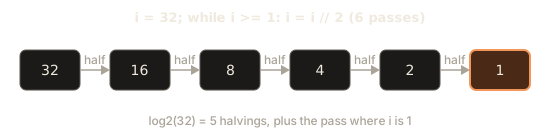
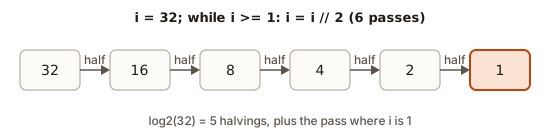 A value halved from 32 down to 1 in six passes
(The base of the logarithm does not matter in Big-O. log10(n) and log2(n) differ by a constant factor, about 3.3, and constants vanish. So we write O(log n) without a base.)
O(n): linear time
Work grows in step with the input. Double the input, double the work. The everyday picture is reading a book: a book twice as long takes twice as long.
A single pass over the data, with constant work per item, is linear. Finding the largest value, summing, counting matches, copying a list and printing every item are all linear.
(1, 9, 35, 4)The loop body does several comparisons and additions, perhaps ten steps per item. Ten times n is still O(n). Doing four jobs in one pass costs no more, in Big-O terms, than doing one. This idea, combining several jobs into one pass, is a practical way to make code faster.
Linear is often the best you can do. If you must look at every item to know the answer, for instance to find the maximum of an unsorted list, you cannot beat O(n) because you cannot skip any item.
O(n log n): linearithmic time
This is the rate of the good sorting algorithms. It lies between linear and quadratic. For a million items, n log n is about 20 million steps, while n^2 is a trillion.
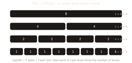
Where does it come from? Merge sort shows it clearly. It splits the list in half, sorts each half, then merges the two sorted halves. Splitting continues until single items remain. The number of levels of splitting is about log n, and each level does about n work for merging. The total is n times log n.
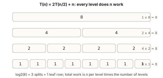 Recursion tree for merge sort on eight items showing eight units of work on each level
Count it by running it. This merge sort counts how many comparisons it makes.
8 17 True
64 306 True
1024 8935 True
16384 208630 True
The comparison counts grow a little faster than n. From 1,024 to 16,384 the input grows 16 times, while the comparisons grow about 23 times, which matches n log n (16 times 14/10 is about 22). For comparison, a quadratic sort would need about 134 million comparisons at 16,384 items, not 208,630.
A useful fact for interviews: any sorting method that works only by comparing pairs of items needs at least about n log n comparisons in the worst case. So O(n log n) is the best you can do for general comparison sorting. Python's built-in sorted and list.sort run in O(n log n).
O(n^2): quadratic time
Work grows with the square of the input. Double the input and the work quadruples. The everyday picture is the handshake problem from the last lesson: every guest greets every other guest.
The code shape is a loop inside a loop where both go over the input.
(3, 21)
10 45
100 4950
1000 499500
For 7 items there are 21 pairs, 7 * 6 / 2. The general count is n(n-1)/2. At n = 1,000 that is 499,500 comparisons; at n = 100,000 it is almost 5 billion. The 1/2 does not change the class: n(n-1)/2 = n^2/2 - n/2, which is O(n^2).
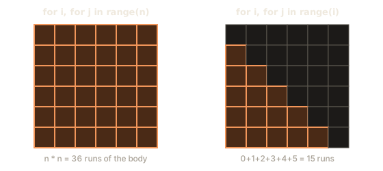
The grid picture shows why. The full double loop visits every cell of an n-by-n square. The version with j starting after i visits only the triangle on one side of the diagonal, about half the cells.
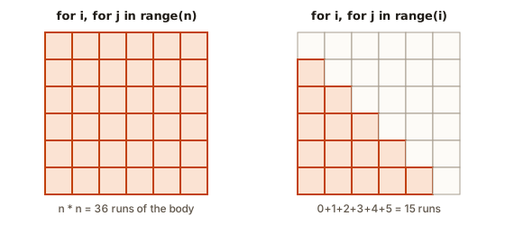 A six by six grid for a full double loop and a triangle for a loop bounded by the outer counter
Simple sorting algorithms, bubble sort, selection sort and insertion sort, are quadratic in the worst case. Step through bubble sort and watch the comparisons pile up.
Outlined bars are being compared. Filled bars were just swapped or written. Bars with a dark border are in their final place. Faded bars are outside the part being worked on.
Compare neighbours and swap them when they are out of order.
Each full sweep bubbles the largest remaining value to the end, and there are about n sweeps of up to n comparisons each. Notice how sweeps get shorter but never fast enough to change the class. After you have watched it, try a reversed list in the visualizer and count the swaps: it is the worst case.
Quadratic code is fine for hundreds or a few thousand items. It is risky for tens of thousands and unusable for millions.
O(n^3): cubic time
Three nested loops over the input give n times n times n. It appears in the textbook method for multiplying two n-by-n tables of numbers (matrices), and in some brute-force searches such as finding three numbers that sum to zero by trying all triples.
(3, 35)
10 120
20 1140
40 9880
Doubling n from 20 to 40 made the work grow from 1,140 to 9,880, a factor of about 8.7, close to the 8 that cubic growth predicts. The triple count is n(n-1)(n-2)/6, still O(n^3). With n = 1,000 that is about 166 million checks, near the limit for one second in a fast language. With n = 10,000 it is hopeless.
The standard improvement for the three-sum problem sorts the list and uses two pointers, giving O(n^2). Knowing a cubic method exists and that a quadratic one beats it is typical interview material.
O(2^n): exponential time
Each time n grows by one, the work doubles. This is the territory of brute force over subsets: for every item you decide "in" or "out", and there are 2 * 2 * ... * 2 = 2^n ways to decide.
The everyday picture is packing a bag from n items, where each item either goes in or stays home. Ten items give 1,024 different bags. Twenty give over a million. Fifty give over a quadrillion, more than you can ever check.
8
[]
['a']
['b']
['a', 'b']
['c']
['a', 'c']
['b', 'c']
['a', 'b', 'c']
5 32
10 1024
20 1048576
Each new item doubles the list of subsets: it keeps all existing subsets and adds a copy of each with the new item. Three items give 8; twenty give 1,048,576.
Exponential algorithms are only usable for small n, up to roughly 20 to 25 in one second. A naive recursive Fibonacci function is a classic accidental example. It looks innocent and is badly slow.
10 55 177
20 6765 21891
25 75025 242785
30 832040 2692537
Each increase of n by 5 multiplies the calls by about 11, so the growth is close to 1.6^n, exponential. At fib(50) this function would make about 40 billion calls. The cure, remembering results already computed, is the subject of the dynamic programming module. It turns the same function into O(n).
O(n!): factorial time
n! is "n factorial", n * (n-1) * (n-2) * ... * 1. It counts the ways to arrange n items in a row. Three items can be ordered 6 ways, ten items 3,628,800 ways. Brute-force search through all orderings, such as trying every route for a delivery driver who must visit every town once, is factorial.
[1, 2, 3]
[1, 3, 2]
[2, 1, 3]
[2, 3, 1]
[3, 1, 2]
[3, 2, 1]
4 24
6 720
8 40320
Factorial grows faster than exponential. Eleven items already give nearly 40 million arrangements; at 20 items the count is about 2.4 quintillion. Programs of this kind work for n up to about 10, perhaps 11. Real route-planning software avoids this by using smarter methods and accepting "very good" instead of "perfect" answers.
Comparing the rungs with numbers
Seeing the numbers together makes the ladder concrete. The next program prints how many steps each class needs for several values of n.
     n |          log n |              n |        n log n |            n^2 |            n^3
    10 |              3 |             10 |             33 |            100 |           1000
   100 |              7 |            100 |            664 |          10000 |        1000000
  1000 |             10 |           1000 |           9966 |        1000000 |     1000000000
 10000 |             13 |          10000 |         132877 |      100000000 |  1000000000000
2^10 = 1024
2^30 = 1073741824
2^60 = 1152921504606846976
20! = 2432902008176640000
Read down the n^3 column: at 10,000 items it is a trillion. Read down log n: the answer stays under 15. The gap between n log n and n^2 at 10,000, 133 thousand against 100 million, is the difference between a blink and a coffee break. And 2^60 is already a number with 19 digits.
Two rungs we skipped: square roots and two inputs
Two other shapes appear often enough to name.
O(sqrt n) sits between O(log n) and O(n). It shows up when a loop stops at the square root, as in the faster prime test of the last lesson. For n = one million the square root is 1,000. A related trick is the divisor listing: to find all divisors of n you only walk d up to the square root, and each hit gives two divisors, d and n // d.
[1, 2, 3, 4, 6, 9, 12, 18, 36]
[1, 97]
240
For 720,720 the loop makes only 849 passes, instead of 720,720, yet it finds all 240 divisors. Notice the check d != n // d: for a perfect square like 36, the divisor 6 pairs with itself and must be listed once.
Two-variable classes appear whenever there are two independent inputs. Merging two sorted lists of lengths a and b is O(a + b). Searching for each of q queries in a sorted list of p items by binary search is O(q log p). Walking a grid of r rows and c columns is O(r * c). Keep the letters separate until the problem tells you how they relate. If the grid is square, r and c are both about the square root of the cell count, and the walk is linear in the number of cells.
How to estimate a logarithm without a calculator
You will often need log2 of a number in your head. Use the powers of two table. These are worth memorising.
| Power | Value |
|---|---|
2^10 | 1,024 (about a thousand) |
2^20 | 1,048,576 (about a million) |
2^30 | 1,073,741,824 (about a billion) |
2^40 | about a trillion |
To get log2(n), find the nearest power of two. For 5,000, we know 2^12 = 4096 and 2^13 = 8192, so log2(5000) is between 12 and 13, about 12.3. For 3 million, 2^21 is about 2 million and 2^22 about 4 million, so log2 is about 21.5.
You can also count digits. Each factor of 1,000 adds about 10 to the logarithm. So a thousand is 10, a million is 20, a billion is 30. That is enough for estimating n log n: a million items cost about 20 million steps.
Python can confirm your estimates.
5000 12.29 13
3000000 21.52 22
1000000000 29.9 30
The bit_length() method returns the number of binary digits, which is floor(log2(n)) + 1. It is a quick way to get the number of halvings a loop will make.
Operation costs of Python's own containers
You will constantly use lists, dictionaries and sets. Knowing their costs saves you from hidden quadratic code. The table gives typical costs, where n is the number of items stored.
| Operation | list | dict | set |
|---|---|---|---|
| read by position or key | O(1) | O(1) average | not applicable |
x in c | O(n) | O(1) average | O(1) average |
| append or add | O(1) amortised | O(1) average | O(1) average |
| insert or delete at the front | O(n) | not applicable | not applicable |
| delete by value | O(n) | O(1) average | O(1) average |
| loop over all | O(n) | O(n) | O(n) |
| sort | O(n log n) | not applicable | not applicable |
Two terms need a note. "Average" means that with typical data the cost is constant, though a rare unlucky data set can make it worse; hash tables later in the course explain when. "Amortised" means averaged over many operations, which is lesson four.
A short experiment shows the cost of a front insert. We count element moves rather than seconds so the output is stable.
10 45 0
100 4950 0
1000 499500 0
The first column is n, the second the number of shifts for front inserts, which equals n(n-1)/2, and the third is always 0 for appends. Inserting at the front n times costs a quadratic number of moves; appending costs none.
Choosing an algorithm from the constraints
Here is how practitioners use the ladder. Problems come with a limit on n and a time limit. A reasonable rule: a fast language does about 10^8 simple steps per second. Python does about 10^7 simple operations per second, so scale accordingly. For a one-second budget in a fast language:
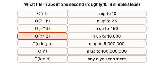 Largest input size each growth rate handles in about one second
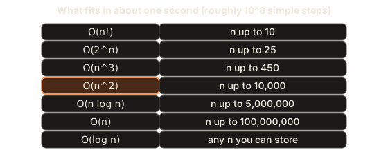
| Limit on n | Complexity you can afford |
|---|---|
| up to 10 | O(n!) or anything |
| up to 20 to 25 | O(2^n) |
| up to 450 | O(n^3) |
| up to 5,000 to 10,000 | O(n^2) |
| up to 1,000,000 | O(n log n) or O(n) |
| up to 10^9 or more | O(log n) or O(1) |
Read the table as a guide, not a law. Constants matter at the borders, and the numbers suggest which method to try first.
Consider an example. A problem says: "You get n up to 200,000 numbers. Find whether any two sum to a given target." The quadratic method does 2 * 10^10 steps, hundreds of seconds. You need O(n log n) or O(n). One answer: put the numbers in a set and, for each x, look up target - x. That is O(n).
True
False
False
Trace the first call. seen starts empty. x = 8: is 14 - 8 = 6 in seen? No. Add 8. x = 3: is 11 in seen? No. Add 3. x = 11: is 14 - 11 = 3 in seen? Yes. Return True. The third call has 200,000 even numbers and an odd target; it needs 200,000 iterations, about a fifth of a second in Python, and finds no pair because two even numbers cannot sum to an odd one. The quadratic method would take hours on it.
Three problems, three decisions
Practise the skill of reading constraints with three short cases. For each one, decide what rung you can afford before writing a line of code.
Case 1: the leaderboard. A game has up to 100,000 players with scores. You must print the top 10. Sorting everything costs O(n log n), about 1.7 million steps: fine. But you do not need a full sort. One pass that keeps the ten best seen so far costs O(n * 10), which is O(n). Both pass the time limit, so choose the one that is simpler to get right. In Python that is sorted(scores, reverse=True)[:10], a single line. The rung tells you that the lazy method is acceptable, which is useful knowledge: you do not have to optimise everything.
Case 2: the group chat. A chat app has up to 3,000 friends and wants every pair of friends who share at least one hobby. Checking all pairs is 3000 * 2999 / 2, about 4.5 million pairs. Each pair compares two short hobby lists. That is well inside the budget, so a nested loop is fine. The same code for 300,000 users would need 4.5 * 10^10 pair checks, and you would invert the idea: for each hobby, list the people who have it, and pair people only within a hobby.
Case 3: the route. A courier must visit 12 addresses and return home, and you must find the shortest route. Trying every order is 12!, about 479 million routes, each needing 12 additions to score. That is about 5.7 billion steps: too slow in Python and borderline in C++. A smarter method, dynamic programming over subsets, costs about n^2 * 2^n, which is 144 * 4096, about 590,000 steps. This is why exponential, not factorial, is the target for the famous travelling-salesman problem on small inputs.
The pattern in all three: write down n, look up the budget, then pick the simplest algorithm that fits. Simpler code has fewer bugs. Reach for the cleverer algorithm only when the budget forces it.
A last experiment shows the decision in numbers. Given a size and a speed in steps per second, which classes finish in under a second?
1000 ['O(log n)', 'O(n)', 'O(n log n)', 'O(n^2)']
100000 ['O(log n)', 'O(n)', 'O(n log n)']
3000000 ['O(log n)', 'O(n)', 'O(n log n)']
At 1,000 items quadratic code still fits, with 10^6 steps, but cubic code does 10^9 steps, ten times over the budget, so it drops out. At 100,000 items quadratic code needs 10^10 steps and also drops out, leaving the three lower rungs. The function ignores constants, so treat a class that is just under the line as a risk, not a promise.
What happens inside: why the classes differ so much
It is worth understanding why the ladder is so steep and why hardware does not rescue you.
Suppose a computer does one billion steps per second, and then you buy a machine ten times faster. For an O(n) algorithm, the largest n solvable in a fixed time grows tenfold. For O(n^2), it grows by only a factor of about 3.2, the square root of 10. For O(2^n), it grows by an additive 3.3: if you could solve n = 40 before, you can solve n = 43 now. A tenfold faster machine buys you three more items. That is the practical meaning of exponential growth. Only a better algorithm helps.
A second reason is memory behaviour. A linear scan over an array is friendly to the processor's cache, the small fast memory next to the processor that holds recently used data. Moving through neighbouring cells in order is fast. Jumping randomly around a huge structure is slow because each jump may need the slow main memory. Two algorithms with the same Big-O can differ by a factor of ten or more for this reason. That is why a plain array often beats a fancier structure at small and medium sizes. Big-O tells you the shape; the constants still decide close races.
Common mistakes
Mistake 1: reading O(n log n) as O(n) * O(log n) and being unsure which is bigger. It is bigger than O(n) and smaller than O(n^2). For all practical n, log n is a small number, 20 for a million and 30 for a billion. So O(n log n) behaves like "linear with a modest multiplier".
Mistake 2: assuming every loop is linear. A loop that multiplies its counter (i *= 2) is logarithmic. A loop whose counter moves by i += i doubles it and is logarithmic. A loop while d * d <= n is O(sqrt n). Look at how the counter changes, not just that a loop exists.
Mistake 3: treating a nested loop as automatically quadratic. If the inner loop runs a fixed 3 times, the pair is O(n). If the inner loop shrinks, as in for j in range(i), the total is still quadratic because 0 + 1 + ... + (n-1) = n(n-1)/2. If the inner loop halves, as in while j > 0: j //= 2, the pair is n log n. Count the total body executions.
Mistake 4: forgetting that sorting costs n log n. A function that calls sorted and then loops once is O(n log n), not O(n). The sort dominates.
Mistake 5: calling something O(1) because a built-in does it in one line. max(items) is one line and O(n). x in some_list is one expression and O(n). some_list.insert(0, x) is one call and O(n), since every item shifts right. text += "x" in a loop can be O(n^2) overall, because each concatenation copies the string. The cost of a line is the cost of what it hides.
Mistake 6: using exponential recursion without noticing. If a recursive function calls itself twice with a slightly smaller input, as fib does, count the calls. Doubling at every level means exponential.
Real error messages for this lesson. Slow algorithms show up in tools in two forms. In an online judge or a test run you see:
Time Limit ExceededIt means your program did not finish within the allowed time. The usual cause is a complexity one rung too high for the input. Check n against the table above before you start micro-optimising.
In Python, deep recursion produces this error instead:
RecursionError: maximum recursion depth exceeded in comparisonPython limits the stack depth, about 1,000 calls by default. A recursive function that goes n levels deep for n = 100,000 fails with this error long before time becomes the problem. Space complexity in the next lesson explains why.
If you accidentally write an infinite loop, the program simply hangs and you stop it with Ctrl+C, which prints:
KeyboardInterruptA debugging walkthrough: the search that got slower every week
A small shop has a function that checks whether a product code is already in use. It was written when the shop had 200 products.
1000Now the shop has 200,000 products and 100,000 queries a day. The program takes minutes. Diagnose it like this.
- Say what n is. There are
pproducts (the catalog) andqqueries. - Find the loops. One visible loop over queries: q passes.
- Find the hidden loop.
q in catalogscans a list: up to p steps. - Multiply. About
q * p: 100,000 times 200,000 is 2 * 10^10, tens of seconds to minutes in Python. The complexity is O(q * p). - Choose a better structure. A set finds membership in about one step. Build it once, which costs O(p), then do q lookups of O(1) each: O(p + q) total.
1000The answer is identical, 1,000, and the cost dropped from O(p * q) to O(p + q). It is the same idea as the duplicate-check example in the last lesson. Spotting list membership inside a loop is one of the most valuable skills in everyday performance work.
Where this shows up in real life and interviews
Databases. A table with no index is a list: finding a row by value scans all rows, O(n). An index is a tree or hash structure that finds it in O(log n) or O(1). Adding an index to a slow query is binary search in disguise.
Search and sorting. Sorting a million records, O(n log n), is quick. Comparing every pair of records, O(n^2), is not. Systems that detect duplicate photos or similar documents work hard to avoid the quadratic pairwise comparison.
Games and graphics. A game that checks every object against every other object each frame is O(n^2) and drops frames at a few thousand objects. Engines divide the world into grids or trees so each object is only compared with neighbours.
Interviews. The common pattern is: first state the brute force and its complexity, then improve it. "Brute force is O(n^2) by checking all pairs. I can sort first, O(n log n), then use two pointers, O(n)." Naming the rungs fluently shows you can compare approaches.
Practice
1. (Easy) Match each snippet to a class: O(1), O(log n), O(n), O(n^2).
# A
return items[len(items) // 2]
# B
for x in items: total += x
# C
i = n
while i > 1: i //= 2
# D
for x in items:
    for y in items: pass
Solution
A is O(1): one read at a computed position. B is O(n): one pass. C is O(log n): i halves each time. D is O(n^2): n passes of n.
2. (Easy) About how many comparisons does binary search need for a sorted list of 1,000,000 items?
Solution
At most floor(log2(1,000,000)) + 1, which is 20. Since 2^20 = 1,048,576 is just above a million, 20 halvings are enough to reduce the range to one item.
3. (Easy) How many subsets does a set of 12 items have? How many orderings does a row of 6 items have?
Solution
Subsets: 2^12 = 4096. Orderings: 6! = 720.
4. (Medium) What is the complexity of this function? Count the body executions for n = 8.
def f(n):
    count = 0
    for i in range(n):
        j = 1
        while j < n:
            count += 1
            j *= 2
    return count
Solution
The inner loop doubles j: 1, 2, 4 for n = 8, so 3 passes. The outer loop runs 8 times. Total 24. In general it is n * ceil(log2(n)), so O(n log n).
24 102405. (Medium) A problem gives n up to 50,000 and a one-second limit in a fast language. Is an O(n^2) solution acceptable? What about O(n log n)?
Solution
50,000^2 = 2.5 * 10^9, about 25 seconds at 10^8 steps per second: too slow. n log n is about 50,000 * 16 = 800,000, far under budget. Look for an O(n log n) idea, such as sorting first or using a hash set.
6. (Medium) What is the complexity of this function, and why?
def f(items):
    items.sort()
    for i in range(len(items) - 1):
        if items[i] == items[i + 1]:
            return True
    return False
Solution
The sort is O(n log n) and the loop is O(n). Sequential parts add, so n log n + n, which is O(n log n). This is the sorted-neighbours method for finding duplicates. It uses less extra memory than a set but changes the input list as a side effect, because sort works in place.
7. (Medium) Count how many times count += 1 runs, as a formula, then name the class.
for i in range(n):
    for j in range(i, n):
        count += 1
Solution
For i = 0 the inner loop runs n times, for i = 1 it runs n - 1 times, and so on down to 1. The sum is n + (n-1) + ... + 1 = n(n+1)/2. That is n^2/2 + n/2, so O(n^2).
8. (Hard) The function below is correct. Give its complexity and a faster version.
def most_frequent(items):
    best = None
    best_count = 0
    for x in items:
        c = items.count(x)
        if c > best_count:
            best_count = c
            best = x
    return best
Solution
items.count(x) is O(n) and it runs n times: O(n^2). Count with a dictionary in one pass:
3Now it is O(n) time and O(k) extra space where k is the number of distinct values.
9. (Hard) A naive fib(40) makes about 331 million calls. Using the table of rungs, explain roughly how long fib(50) would take compared with fib(40), given that growth is close to 1.6^n.
Solution
Ten more steps multiply the work by about 1.6^10, which is about 110. So fib(50) needs roughly 110 times the calls of fib(40): about 36 billion. If fib(40) took 30 seconds in Python, fib(50) would take close to an hour. Exponential growth turns a modest increase in n into a huge increase in time.
10. (Hard) Your program has a loop over n items. Inside it you call a helper that sorts a fresh copy of a 100-item list. What is the complexity in terms of n?
Solution
The helper's list has a fixed size of 100, so each sort costs a constant number of steps (about 100 * 7). It runs n times, so the total is O(n) with a big constant. This is a good example of why "sort inside a loop" is not automatically bad: what matters is whether the sorted size depends on n. If the helper sorted all n items, the total would be O(n^2 log n).
What you now know
- The standard ladder, from slow growth to fast growth, is O(1), O(log n), O(n), O(n log n), O(n^2), O(n^3), O(2^n), O(n!).
- Halving or doubling a loop variable gives log n, one pass gives n, a pass inside a pass gives n squared, and trying every subset or ordering gives 2^n or n!.
- About 10^8 simple steps fit in one second in a fast language, so the size limit on n tells you which class to aim for.
- Built-in calls hide loops:
inon a list,count,sort,insertat the front and string concatenation all cost more than one step. - Faster hardware does not rescue a bad class; a better algorithm or data structure does.