Why it matters
Many tree questions ask for an answer "per level" or "as seen from one side". A company chart might ask for the managers at each rank. A map might ask what you see when you stand on the left of a building. A network planner asks for the number of hops at each distance from the router. All of these start from the same tool, a level-order walk with a queue, and then add one small rule. Interviewers use these questions to check that you can keep a queue straight and reason about a picture.
This lesson builds the level walk from first principles, then turns it into five views. Each view changes only one line of the basic code, which is the point: a good pattern makes many questions short.
The idea: a queue visits one level at a time
A queue is a line of people waiting for service. New people join at the back, and the front person is served first. In C++ a queue is std::queue, with push to add at the back, front to read the first item, and pop to remove it. The order is first in, first out.
Level order uses a queue as follows. Put the root in the queue. Then repeat: take the front node out, visit it, and add its children to the back. Because children always go behind everything already waiting, all nodes of one level leave the queue before any node of the next level.
Here is that process on the tree from the earlier lessons, 1 2 3 4 5 -1 6:
        1
       / \
      2   3
     / \   \
4 5 6| Step | Node taken from the front | Children added to the back | Queue after the step |
|---|---|---|---|
| 0 | none | none | 1 |
| 1 | 1 | 2, 3 | 2, 3 |
| 2 | 2 | 4, 5 | 3, 4, 5 |
| 3 | 3 | 6 (3 has no left child) | 4, 5, 6 |
| 4 | 4 | none | 5, 6 |
| 5 | 5 | none | 6 |
| 6 | 6 | none | empty, stop |
The visit order is 1, 2, 3, 4, 5, 6. That is one flat list, and it does not show the levels. To keep the levels separate, you need one more idea.
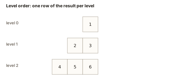 Each row of the picture is one level of the tree, drawn as boxes with the nodes of that level inside
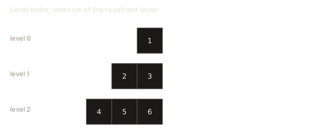
Taking a snapshot of the queue size
At the start of a round, the queue holds exactly the nodes of the current level. Their children have not been added yet. So if you read q.size() at the start of the round, that number is the count of the current level. Process exactly that many nodes, and their children join the back of the queue as the next level. Then start the next round.
while (!q.empty()) {
    int sz = q.size();          // the number of nodes on this level
    for (int i = 0; i < sz; i++) {
        TreeNode* n = q.front();
        q.pop();
        // visit n, add its children to the back
    }
    // the queue now holds exactly the next level
}
The snapshot sz is the key. If you wrote i < q.size() in the loop condition instead, the number would change on every step, because the loop pops nodes and pushes children. The loop would then process the children of the current level as well, and the levels would blur together. This is the most common bug in level-order code, and the next section shows what it looks like in practice.
Level order grouped by level
The next program turns the snapshot idea into a function. It returns a vector of rows, one row per level. The first row is the root, the second row holds the root's children, and so on.
Type 1 2 3 4 5 -1 6 into the Input box and click Run.
1
2 3
4 5 6
Trace the first round. The queue starts with the root, so sz is 1. The inner loop takes 1 out, adds 1 to the row, and pushes its children 2 and 3. The row [1] is saved, and the queue is now 2, 3.
The second round reads sz = 2. It takes 2 out and pushes 4 and 5, then takes 3 out and pushes 6. The row is [2, 3], and the queue is 4, 5, 6. The third round reads sz = 3, takes out all three, and pushes nothing, since they are leaves. The row is [4, 5, 6], and the queue is empty, so the loop ends.
Time is O(n), because each node enters and leaves the queue once. Space is O(w), where w is the width of the widest level, because the queue never holds more than one level plus the children of the nodes taken out. For a perfect tree of height h, the widest level holds about n/2 nodes, so the space is still O(n) in that case.
empty
removed: nothing
Items leave from the front and join at the back. An outlined box was just added or peeked.
The queue is empty. The first item added is the first one removed.
Use the queue visualizer above to watch the snapshot at work. Each round removes exactly the number of nodes that were waiting at its start, and the children of those nodes wait at the back for the next round.
Left view and right view
The right view of a tree is what you see when you stand on its right side. It is the rightmost node of every level. The left view is the leftmost node of every level. Both are easy with the levels function, because each row already lists its nodes from left to right.
The first node of each row is the left-most one, and the last is the right-most one. Here is the code. It reuses levels, build and printRow from the program above, so only the new function is shown in the explanation; the full program follows.
vector<int> leftView(const vector<vector<int>>& rows) {
    vector<int> out;
    for (auto& row : rows) out.push_back(row.front());
    return out;
}

vector<int> rightView(const vector<vector<int>>& rows) {
    vector<int> out;
    for (auto& row : rows) out.push_back(row.back());
    return out;
}
Notice that the left view of the example tree is 1, 2, 4, and the right view is 1, 3, 6. The value 5 is not in the left view, because 4 stands before it on its level. It is not in the right view either, because 6 is last on its level. The views depend on the level, not only on whether a node is a left or right child.
Here is the full program. It prints both views for the input in the box.
left view: 1 2 4
right view: 1 3 6
Check the output against the picture. Level 0 is [1], so both views start with 1. Level 1 is [2, 3], so the left view takes 2 and the right view takes 3. Level 2 is [4, 5, 6], so the left view takes 4 and the right view takes 6.
Time is O(n) for the walk and the views, and the extra space is O(n) for the rows.
Top view and bottom view
The top view is what you see when you look down on the tree from above. Each node sits at a horizontal distance from the root. The root has distance 0, a left child has one less than its parent, and a right child has one more. Looking from above, you see for each distance the node that is highest in the tree, because the higher node hides the lower ones beneath it. The bottom view is the opposite: for each distance, you see the lowest node.
The algorithm is a level-order walk that carries the horizontal distance with each node. A map from distance to value keeps the answer. For the top view, the map keeps the first value it sees for each distance, because level order meets higher nodes first. The map keeps its keys in sorted order, so reading it from the first key to the last gives the view from left to right.
The bottom view is the same, except that the map is overwritten every time a node is seen at a distance. Since level order goes from the top down, the last node written for each distance is the lowest.
Here is the program. It prints the top and bottom views of the input tree.
top view: 4 2 1 3 6
bottom view: 4 2 5 3 6
Walk through the distances for the example tree. Node 1 has distance 0. Node 2 is its left child, so distance -1, and node 3 is its right child, so distance 1. Node 4 is the left child of 2, so its distance is -2. Node 5 is the right child of 2, so its distance is -1 + 1 = 0. Node 6 is the right child of 3, so its distance is 1 + 1 = 2.
For the top view, distance -2 holds 4, distance -1 holds 2, distance 0 is first reached by 1 (level 0), and node 5 at distance 0 is later and is ignored. Distance 1 holds 3, and distance 2 holds 6. The output is 4 2 1 3 6.
For the bottom view, distance 0 is overwritten by 5, which is on a lower level. The output is 4 2 5 3 6.
Notice what the top view shows. Node 5 is hidden by node 1 when you look from above, because 1 is higher at the same distance. Node 4 is visible, because no node sits above it at distance -2.
The map costs O(log k) for each insert, where k is the number of distances. So the total time is O(n log n). The space is O(n) for the queue and the map.
Zig-zag level order
A zig-zag level order reads the first level left to right, the second level right to left, the third left to right, and so on. It is a common question, and it needs just one change to the levels function: after building each row, reverse it when its level number is odd. Level numbers count from 0 at the root.
void zigzagFix(vector<vector<int>>& rows) {
    for (size_t d = 1; d < rows.size(); d += 2) {
        reverse(rows[d].begin(), rows[d].end());
    }
}
The loop starts at level 1 and skips every other row. For the example tree, the rows are [1], [2, 3], [4, 5, 6]. After the fix, row 1 becomes [3, 2], and row 2 is left alone. The output is 1, then 3 2, then 4 5 6.
Here is the complete program. Type 1 2 3 4 5 -1 6 into the Input box and click Run.
1
3 2
4 5 6
Per-level sums and maxima
Once the rows exist, most per-level questions are a few lines over them. The next program computes two of them, the sum and the maximum of every level. It keeps the same levels function, and the new work happens in main. Type 1 2 3 4 5 -1 6 into the Input box and click Run.
sums: 1 5 15
maxes: 1 3 6
The sum of level 2 is 4 + 5 + 6, which is 15. The maximum of level 1 is 3, because the row is 2 3. The sums use long long, so a wide level with large values cannot overflow. Each row is independent of the others, so the program is one simple loop per question. That is the point of building the rows first: once a level is a vector, any question about it is one short loop.
Notice that max_element needs a nonempty row. Every row of levels has at least one value, because a level is only added when a node exists, so this is safe. If you ever build rows by hand, check for an empty row first.
Depth tags: an alternative to the snapshot
The snapshot of the queue size is not the only way to separate levels. The second method stores the depth of each node next to the node in the queue. When a node is taken out, its depth tells you which row it belongs to. A new row starts when the depth is one more than the number of rows so far.
vector<vector<int>> rows;
queue<pair<TreeNode*, int>> q;
q.push({root, 0});
while (!q.empty()) {
    auto [n, d] = q.front();
    q.pop();
    if (d == (int)rows.size()) rows.push_back({});
    rows[d].push_back(n->val);
    if (n->left) q.push({n->left, d + 1});
    if (n->right) q.push({n->right, d + 1});
}
Both methods give the same rows. The depth-tag method is handy when you need the depth for another purpose, for example to compute a horizontal distance, as the top view does. The snapshot method is shorter when you only need the rows, and it uses less memory per queue entry, because it stores only the node pointer. Learn both, and say which one you chose and why.
The rule for the depth-tag version is that the queue is always in depth order. Nodes of depth d are all in front of nodes of depth d plus one, because each node adds its children at the back. So the first node you see at a new depth is the first node of its row, and rows.size() grows by exactly one each time a new depth begins.
Tracing the top view step by step
The top view from earlier in this lesson is a good place to see the queue and the map work together. Here is a full trace for the input 1 2 3 4 5 -1 6. Each row shows the node taken from the queue, its horizontal distance (hd), the map after the step, and the nodes pushed.
| Step | Node taken (hd) | Map after the step | Pushed to the back |
|---|---|---|---|
| 1 | 1 (0) | {0: 1} | 2 (hd -1), 3 (hd 1) |
| 2 | 2 (-1) | {-1: 2, 0: 1} | 4 (hd -2), 5 (hd 0) |
| 3 | 3 (1) | {-1: 2, 0: 1, 1: 3} | 6 (hd 2) |
| 4 | 4 (-2) | {-2: 4, -1: 2, 0: 1, 1: 3} | nothing |
| 5 | 5 (0) | no change, hd 0 is already set | nothing |
| 6 | 6 (2) | {-2: 4, -1: 2, 0: 1, 1: 3, 2: 6} | nothing |
The map is printed from its smallest key to its largest, which gives 4 2 1 3 6. Step 5 is the important one. Node 5 sits at hd 0, but the map already holds 1 for that key, so the count check skips it. Node 1 is higher in the tree, and it is the one you see from above. Node 5 is hidden beneath it.
Compare this with the bottom view. The bottom view overwrites the map at step 5, so hd 0 becomes 5, and the output changes to 4 2 5 3 6. The only difference between the two views is one line of code, and the trace shows exactly where it matters.
Worked example: a level with a missing middle
Level order has a subtle property that trips people up. A level can have gaps, and the rows still list only the real nodes. Take the input 1 2 3 -1 4 -1 5. Read it level by level: the root 1 has children 2 and 3. Node 2 has a left child missing and a right child 4. Node 3 has a left child missing and a right child 5. The levels are 1, then 2 3, then 4 5. The output of the rows is:
1
2 3
4 5
Notice that 4 is a right child, yet it is the first value in its row, because nothing on its level sits to its left. The row shows the real nodes in left-to-right order, and it never shows the gaps. So the left view takes 4 for level 2, and the right view takes 5. The top view is different, because it depends on horizontal distance. Node 2 has distance -1, so node 4 has distance 0, the same as the root, and node 5 has distance 2. The top view is therefore 2 1 3 5, with 4 hidden under the root.
Worked example: one seven-node tree in every view
Before you move on, run the whole family of views on one tree, so that you can compare them side by side. Take the input 10 4 15 2 -1 -1 20. Read it level by level: the root is 10, its children are 4 and 15, node 4 has a left child 2 and no right child, and node 15 has no left child and a right child 20. Draw it before you read on:
        10
       /  \
      4    15
     /       \
    2         20
The rows are 10, then 4 15, then 2 20. Every view below is built from these rows, or from the horizontal distances that the top and bottom views use. The outputs are the ones the programs in this lesson print for this input.
levels:
10
4 15
2 20

left view: 10 4 2
right view: 10 15 20

top view: 2 4 10 15 20
bottom view: 2 4 10 15 20

zig-zag:
10
15 4
2 20
Check the two views that come from rows. The left view takes the first value of each row, so 10, 4 and 2. The right view takes the last, so 10, 15 and 20. The zig-zag order reverses only the middle row, because the middle row is the odd one, so it reads 15 4.
Now the views that use horizontal distance. The root is at 0, so 4 is at -1 and 15 is at 1. Node 2 is the left child of 4, so it is at -2. Node 20 is the right child of 15, so it is at 2. Every distance holds exactly one node, so the top view and the bottom view are the same, and both print 2 4 10 15 20. Pick a tree where a distance holds two nodes, such as the example in the earlier section, to see the two views differ.
Two lessons follow from this tree. First, the left and right views and the zig-zag order use the rows and nothing else, so a wrong row gives wrong answers for all three at once. Second, the top and bottom views use distances and nothing else, so a wrong distance gives a wrong answer for one view and not always the other. When a view is wrong, first ask whether its rows or its distances are wrong. The answer tells you which function to read.
Reading rows back into a picture
Going the other way is a useful interview habit. Given a list of rows, you should be able to draw the tree that produced them, at least when each level is complete. If the rows are 1, 2 3, 4 5 6 7, the tree is perfect with four levels, and its left view is 1, 2, 4. If the rows are 1, 2 3, 4 5, then the tree has a last level that is only partly full, and you must choose where the gaps are. The rows alone do not tell you where the children are, so a row list does not define a unique tree. Say so, and ask for the level-order list with -1 markers if the question needs one exact tree.
This is why the level-order input format has -1 markers. Without them, the same rows could describe many different trees, and the input would be ambiguous.
Edge cases
- The empty tree.
levels(nullptr)returns no rows, so every view prints nothing. The left and right view code loops over zero rows and never readsrow.front(), which is why the check at the top oflevelsmatters. - One node. There is one row with one value, so the left view, right view, top view and bottom view all print that value.
- A skewed tree. Each row has one node. The zig-zag order is the same as the plain order, because reversing a row with one value changes nothing. The left and right views are identical, and both equal the whole tree read top to bottom.
- A partial last level. The last row has fewer nodes than the one above it, and it may have gaps in the tree shape. The rows still list only the real nodes, as shown above.
- A tree with values that repeat. The rows and the views still work, because they store values, not pointers. The top view with a map keyed by horizontal distance is not affected by repeated values, because the key is the distance, not the value.
Variations you will meet
- Average per level. Sum the row as a
double, then divide by the row size. The lesson's exercise asks for it. - The level with the largest sum. Compute the sum of each row, then return the index of the first row that has the largest sum. Choose the first one on a tie, and say so in the answer, because a tie without a rule is ambiguous.
- Number of nodes at distance k. The answer is the size of row k, or 0 if the tree is shallower than k. This is the answer to "how many people are k steps from the root?"
- Bottom view and right view together. The bottom view keeps the last node at each horizontal distance, and the right view keeps the last node at each level. Both are "last seen" rules. They differ in the key: distance for the bottom view, and level for the right view.
- Boundary of a tree. Print the left edge going down, then the leaves left to right, then the right edge going up. It mixes the left view, the leaves and the right view, and it is a common follow-up question.
What happens inside the queue
It helps to picture the queue at the start of each round. The queue holds the nodes of the current level that have not been processed yet. As the round takes nodes from the front, it adds their children to the back. So during a round the queue holds two groups: the unprocessed rest of the current level, followed by the children of the nodes already processed in this round.
At the start of round d, the queue holds exactly the nodes of level d. Those are the sz nodes, and the round processes all of them. During the round, the queue holds the part of level d that has not been taken out yet, plus the children of the nodes already taken out in this round. So its size can reach the width of level d plus the width of level d plus one, which is at most twice the widest level. The space is O(w), where w is the widest level.
Interview follow-ups
- Why not use recursion for the rows? You can, by passing the depth down and appending to
rows[depth], but the order of the output is then the order of the walk, not the order of the levels. That still works, because each node knows its depth. Recursion uses O(h) stack space, and the queue uses O(w). For a wide, shallow tree, the queue can use more memory than recursion. For a skewed tree, recursion can use more stack than the queue. Know both trade-offs. - How do you find the first level that has any node with a certain value? Walk the rows in order and stop at the first row that contains the value. The row index is the level.
- What is the time complexity of the zig-zag order? It is O(n), because the reversal of each row costs the size of that row, and the sum of all row sizes is n.
Common mistakes and their real messages
Using the queue size in the loop condition
The loop for (int i = 0; i < q.size(); i++) looks like it does the same job as the snapshot, but it does not. Each pop shrinks the queue, and each child push grows it again, so the condition changes during the loop. In the example tree, the loop keeps going while the queue grows. It takes 1 and pushes 2 and 3, so the condition sees a size of 2, and it takes 2 and pushes 4 and 5, and so on. The first row comes out as 1, 2, 3 instead of 1, and every later row is shifted. The fix is the snapshot: save int sz = q.size(); before the inner loop, and loop to sz.
Forgetting to include the map header
The top and bottom views use std::map. If you leave out #include <map>, the compiler reports:
error: 'map' was not declared in this scopeThe fix is to add the include line at the top of the file.
Using structured bindings in an old standard
The line auto [n, hd] = q.front(); is a structured binding, a C++17 feature. If you compile with -std=c++14, the compiler warns:
warning: structured bindings only available with '-std=c++17' or '-std=gnu++17' [-Wc++17-extensions]The programs in this module use g++ -std=c++17, so the warning does not appear. If you see it, add the flag, or write q.front().first and q.front().second instead.
Calling front on an empty queue
If a loop reads q.front() when the queue is empty, the program is in trouble. On this system, the standard library checks the call and aborts the program with this message:
Assertion '!this->empty()' failed.The exit status is 134, which means the program stopped itself with an abort signal. The fix is to make sure the loop checks q.empty() before it reads the front. The inner loop with the snapshot is safe, because it runs only sz times, and each run removes one node. Make sure sz is never larger than the queue, which happens when you change the code and forget the snapshot.
Using depth-first search for a view
It is tempting to write the top view with a recursive walk, passing the distance down. That can give the wrong answer. A depth-first walk may reach a deep node at distance 0 before a shallow node at distance 0, so the first value it stores is not the highest. Level order avoids this, because it reaches every shallow node before any deep one.
Debugging walkthrough
Suppose your levels function prints 1 2 3 as its first row for the example tree. The first row should hold only the root, so the walk took too many nodes in its first round. Here is how to find the cause.
First, look at the shape of the output. The first row has three values, and nodes 2 and 3 belong on the second row. So the round kept going after it had taken out the root. That points at the loop condition.
Second, print the size at each round. Add cout << "round size " << sz << "\n"; after the line that reads sz. For a correct walk the sizes are 1, 2, 3, one for each level. If the number printed changes during a round, the loop is reading the live queue size, and the snapshot is missing or in the wrong place.
Third, check the position of the snapshot. It must come before the inner loop, and it must not be recomputed inside the loop. A line like for (int i = 0; i < q.size(); i++) is the same bug in a different form.
Fourth, fix the code, and then run the three small trees: the empty tree (-1), the one-node tree (1), and a skewed tree (1 2 -1 3). Each should print one row per level, with the correct number of nodes in each row.
Interview questions you should be ready for
- How do you print a tree one level per line? Use a queue, take a snapshot of its size at the start of each round, and process exactly that many nodes.
- What is the space cost of level order? O(w), where w is the width of the widest level, because the queue holds about one level at a time.
- How would you find the average of each level? Use the same walk, and divide the sum of each row by its length. Use a
doublefor the average, so the division does not truncate. - Why does the top view need level order and not depth-first search? Level order reaches the higher node first at each distance, so the first node stored at a distance is the one highest in the tree.
- How many views can one walk give? Many. Each view is the first, last or some chosen node per row or per distance. The walk does the work once, and the choice of rule decides the answer.
Real-world uses
Level order is breadth-first search, the same idea used to find the shortest number of hops in a social network. A web crawler visits pages in level order, so that it finds the close pages before the distant ones. A file explorer that shows the top few levels of a folder uses the same walk. A user interface draws the rows of a menu tree one row at a time. A view that shows only the top of a tree, such as an organization chart as seen from above, is the top view of this lesson.
Practice
- Print the tree in zig-zag order for the input
1 2 3 4 5 -1 6. Predict the three lines before you run the code.
Solution
The output is 1, then 3 2, then 4 5 6. The first row is left to right, the second row is reversed, and the third row is left to right again.
- Return the largest value on each level. For the example tree, the answer is 1, 3, 6.
Solution
vector<int> levelMax(const vector<vector<int>>& rows) {
    vector<int> out;
    for (auto& row : rows) {
        int best = row[0];
        for (int x : row) best = max(best, x);
        out.push_back(best);
    }
    return out;
}
Each row is a complete level, so its maximum is the answer for that level. The function uses max from <algorithm>.
- Write the average of each level as a
double. For the example tree, the averages are 1.0, 2.5 and 5.0.
Solution
vector<double> levelAverages(const vector<vector<int>>& rows) {
    vector<double> out;
    for (auto& row : rows) {
        double sum = 0;
        for (int x : row) sum += x;
        out.push_back(sum / row.size());
    }
    return out;
}
The sum is stored in a double, and the division uses row.size(), which the compiler converts to a double in the division. Without that, the result would be cut to an integer.
- Find the width of the widest level. For the example tree, the width is 3.
Solution
int widestLevel(const vector<vector<int>>& rows) {
    int width = 0;
    for (auto& row : rows) width = max(width, (int)row.size());
    return width;
}
Each row's size is the number of nodes on that level, so the largest size is the width.
- Write the bottom view for the example tree. The answer is 4 2 5 3 6, as shown in this lesson. Explain why 5 wins over 1 at distance 0.
Solution
Node 5 is on level 2, and node 1 is on level 0. The bottom view keeps the value written last for each distance. Level order writes level 0 first and level 2 later, so the write for 5 comes after the write for 1, and 5 overwrites it. The lowest node at that distance is 5.
- Explain why the code
if (!seen.count(hd)) seen[hd] = n->val;is the top view and not the bottom view, and what changes for the bottom view.
Solution
The check !seen.count(hd) is true only the first time a distance appears, so the first node wins. That is the top view. For the bottom view, drop the check and always write seen[hd] = n->val;, so that the last node written at each distance wins.
- Write a function that returns the depth of the first leaf found in a level-order walk. Explain why it is the minimum depth, and compare it with the recursive version from the previous lesson.
Solution
int firstLeafDepth(TreeNode* root) {
    if (!root) return 0;
    queue<pair<TreeNode*, int>> q;
    q.push({root, 1});
    while (!q.empty()) {
        auto [n, d] = q.front();
        q.pop();
        if (!n->left && !n->right) return d;
        if (n->left) q.push({n->left, d + 1});
        if (n->right) q.push({n->right, d + 1});
    }
    return 0;
}
The walk visits shallow nodes before deep ones, so the first leaf it pops has the smallest depth. It stops early, which is faster than a full walk when a leaf sits near the top. The recursive version from the previous lesson checks every path, so it is simpler to read but does more work on some trees.
- Predict the output of the levels function on the input
1 -1 2 -1 3, which is a chain going right. Then check it.
Solution
Each level has one node, so the output is three lines: 1, 2 and 3. The queue holds one node at each round, so every snapshot is 1.
- Write a function that returns true if a tree is complete, meaning every level is full except possibly the last, and the last level fills from the left. Hint: in a level-order walk, once you see a missing child, no later node may have a child.
Solution
bool isComplete(TreeNode* root) {
    if (!root) return true;
    queue<TreeNode*> q;
    q.push(root);
    bool sawGap = false;
    while (!q.empty()) {
        TreeNode* n = q.front();
        q.pop();
        if (!n) {
            sawGap = true;
            continue;
        }
        if (sawGap) return false;     // a node after a gap breaks the rule
        q.push(n->left);
        q.push(n->right);
    }
    return true;
}
The queue here stores null children too, so that gaps are visible. The first null sets sawGap, and any real node after that means the tree is not complete. The answer for 1 2 3 4 5 -1 6 is false, because node 3 has no left child but node 6 is on the same level as 4 and 5, and the gap comes before 6.
- Two-step question. A perfect tree of height 3 (four levels) has 15 nodes. How many rows does a level-order walk produce, and how many values are in the largest row?
Solution
There are four rows, one for each level from 0 to 3. The largest row is the last level, which has 2 to the power 3, which is 8 nodes. The rows have sizes 1, 2, 4 and 8, which add up to 15.
What you now know
- A queue gives first-in, first-out order. Level order puts the root in the queue and takes nodes out, adding children to the back.
- A snapshot of the queue size at the start of each round separates the levels.
- Each row of
levelsis one level from left to right. The left view takes the first of each row, and the right view takes the last. - The top view keeps the first node seen at each horizontal distance, and the bottom view keeps the last. A
mapkeeps the answers in left-to-right order. - Zig-zag order reverses every other row.
- Common bugs are a loop condition that uses
q.size()directly,front()on an empty queue, a missing#include <map>, and a depth-first walk used where level order is needed.