Why it matters
Maps, social networks, course prerequisites and the links between web pages are all graphs. Interviewers use graph questions to see whether you can turn a messy real problem into a clear structure and then walk through that structure without missing anything. This lesson gives you the two basics that every later graph lesson uses: how to store a graph in a program, and how to search it breadth first.
You need to know for loops, vector and queue from earlier modules. If queue is new to you, read the stacks and queues lesson first. You do not need anything else.
Start with a picture
Imagine a small town with five squares. Some pairs of squares are joined by a footpath. Nothing is measured yet. You only know which squares connect to which. Computer scientists call the squares vertices (one of them is a vertex) and the footpaths edges. Together they form a graph.
A graph is not a special kind of drawing. It is a way of saying that things relate to other things. A friend list is a graph where people are vertices and friendships are edges. A list of tasks where "task B needs task A first" is a graph too. Once you see the vertices and edges, you can ask useful questions. Can I get from here to there? What is the fewest steps? Are these two parts of the town cut off from each other?
Three properties decide which method you use.
- Undirected: every edge works both ways. A footpath is like this. You can walk it in either direction.
- Directed: each edge has one direction, like a one-way street or a course prerequisite.
- Weighted: each edge carries a number, such as a length or a price. An unweighted graph is one where every edge counts the same.
The degree of a vertex is the number of edges that touch it. In an undirected graph, a vertex with three footpaths has degree 3. In a directed graph you count incoming and outgoing edges separately. Incoming edges are called the in-degree and you will need that word in the next lesson.
A neighbour of a vertex v is any vertex that shares an edge with v. A path is a sequence of vertices where each step uses an edge. The length of a path, in an unweighted graph, is the number of edges it uses.
We will number the vertices 0 to n - 1. That lets us use a vertex number as an array index, which is the key to storing graphs cheaply. Here n is the number of vertices and e is the number of edges.
Two ways to store a graph
The adjacency matrix
An adjacency matrix is an n by n table. The cell in row a and column b holds 1 when there is an edge from a to b, and 0 otherwise. To check one edge, you look up one cell.
The cost is fixed. A matrix always has n times n cells, even when the graph has almost no edges. For 1,000 vertices that is a million cells. For 100,000 vertices it is ten billion cells, which will not fit in memory on an ordinary computer.
The adjacency list
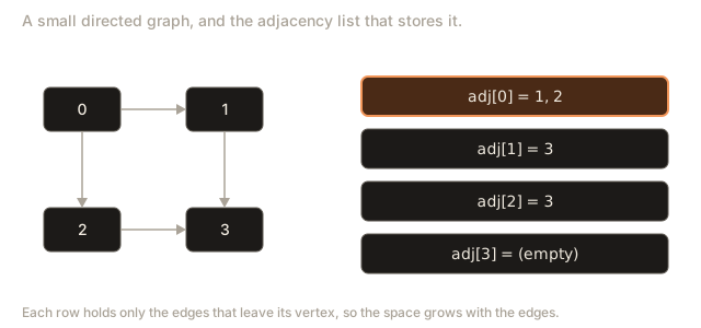
An adjacency list gives every vertex its own list of neighbours. In C++ this is a vector of vectors. The line vector<vector<int>> adj(n); creates n empty lists. The list for vertex v is adj[v], and you add a neighbour with adj[v].push_back(w).
The memory is proportional to n plus e. Each vertex costs one list header, and each edge costs one or two entries. For an undirected edge you store the edge twice: a lists b, and b lists a.
Which one to pick
Here is the comparison as a table.
| Question | Matrix | List |
|---|---|---|
| Memory | n * n cells | about n + e entries |
Is there an edge from a to b? | one lookup | scan adj[a], which costs the degree of a |
Visit all neighbours of v | scan a whole row of n cells | visit only the degree of v |
| Good for | dense graphs, where most pairs are joined | sparse graphs, where few pairs are joined |
Most real graphs are sparse. A social network with a billion users does not have a billion times a billion friendships. Each person has a few hundred friends at most. That is why the list is the default, and why the matrix is only worth its cost for small or very dense graphs.
Picture two ways of keeping track of who knows whom at a party. The matrix is a seating chart with one box for every pair of guests, and most boxes stay blank. The list is a guest book where each guest writes down only the people they know. The guest book is much shorter, and it is the one you would use for a real party with a thousand people.
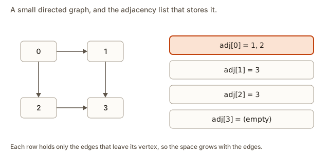 A small directed graph beside its adjacency list
Reading a graph from input
Programs usually get their graph from the keyboard or from a file. The input format in this lesson is simple. The first line holds n and m: the number of vertices and the number of edges. Each of the next m lines holds two numbers a and b, meaning there is an undirected edge between a and b.
The first program reads that input and prints the neighbour list of every vertex.
In the Input box, type these lines exactly. Each line is one line of input:
6 5
0 1
0 2
1 3
2 3
3 4
Click Run. The program prints:
0: 1 2
1: 0 3
2: 0 3
3: 1 2 4
4: 3
5:
Look at each part of the program. cin >> n >> m reads the first line into two variables. vector<vector<int>> adj(n); makes the empty lists. The loop reads one edge per pass. For the edge 0 1, it adds 1 to the list of 0, and it adds 0 to the list of 1. Those two lines are the reason the output shows 0 in the row for 1. The last loop prints each list. Vertex 5 has no edges, so its line ends right after the colon.
Trace the first edge by hand. Before the loop, adj is six empty lists. After reading 0 1, adj[0] is [1] and adj[1] is [0]. After reading 0 2, adj[0] is [1, 2] and adj[2] is [0]. Continue this way for all five edges and you get exactly the printed lists. Working a small case by hand before trusting a program is one of the best habits you can build.
Notice that the order in each list follows the order of the input. The edges 1 3 and 2 3 were read after 0 1 and 0 2, so 3 appears after them in the lists of 1 and 2. The program does not sort the lists. Most graph algorithms do not care about the order, but tests that compare exact output do.
The idea of breadth-first search
Once a graph is stored, the first real task is searching it. The search that visits vertices in rings is called breadth-first search, or BFS.
Start at a chosen vertex, called the source. Visit it. Then visit every vertex one edge away from it. Then every vertex two edges away, and so on. Each ring is finished before the next ring begins. Picture a stone dropped in a pond. The ripples spread out in circles, and each circle is one step further from the stone. BFS works the same way.
A queue is what makes the rings happen. A queue is a line where the first item added is the first item removed, which is called first in, first out (FIFO). You add new vertices at the back and take the next vertex to visit from the front. Because older vertices always leave first, the vertices of one ring are all handled before any vertex of the next ring.
Before the search, step through a plain queue. Notice that the first item added is always the first one removed.
empty
removed: nothing
Items leave from the front and join at the back. An outlined box was just added or peeked.
The queue is empty. The first item added is the first one removed.
BFS keeps a dist array. dist[v] holds the number of edges on the shortest route from the source to v. A value of -1 means the vertex has not been reached yet. When you first reach a vertex from a vertex v, you set its distance to dist[v] + 1 and add it to the queue. You never change a distance after it is set, because the first time you reach a vertex is by the shortest route.
That last point is the heart of the method. The rings grow one edge at a time. A vertex that is reached in ring k cannot be reached in an earlier ring by some other route, because the earlier rings were fully explored first. So the first arrival is always by a path with the fewest edges. In an unweighted graph, BFS gives the shortest paths.
Step through the search below. Watch which vertex leaves the queue at each step, and watch the distances fill in as the rings grow.
A filled node is the one being handled. An outlined node is in the queue. A dark border means visited. The thick dashed edge is the one being looked at. Neighbours are tried in alphabetical order.
Start at A. Put it in the queue.
Look for three things while you step. First, the queue always holds vertices from at most two neighbouring rings. Second, a vertex is added to the queue only once, at the moment it is first reached. Third, the vertex that is never reached keeps distance -1, because no path leads to it from the source.
A worked example by hand
Let us trace BFS on the graph from the first program. The source is 0, and the adjacency lists are the ones printed earlier. Here is the state after each step. The queue is written with its front on the left.
Start: dist[0] = 0, queue [0].
Step 1. Pop 0. Its neighbours are 1 and 2. Neither has a distance yet, so set dist[1] = 1 and dist[2] = 1. Push both. Queue [1, 2].
Step 2. Pop 1. Its neighbours are 0 and 3. Vertex 0 already has a distance, so skip it. Vertex 3 is new: set dist[3] = 2 and push it. Queue [2, 3].
Step 3. Pop 2. Its neighbours are 0 and 3. Both already have distances. Nothing is pushed. Queue [3].
Step 4. Pop 3. Its neighbours are 1, 2 and 4. The first two are done. Vertex 4 is new: set dist[4] = 3 and push it. Queue [4].
Step 5. Pop 4. Its only neighbour is 3, which is done. Queue empty, so the search ends.
Vertex 5 was never pushed, so dist[5] is still -1. Here is the final table.
vertex:  0  1  2  3  4  5
dist:    0  1  1  2  3 -1
This is the same answer the next program prints. Notice the order of the rings: 0 at distance 0, then 1 and 2 at distance 1, then 3 at distance 2, then 4 at distance 3. The rings are visible in the table, and they match the picture below.
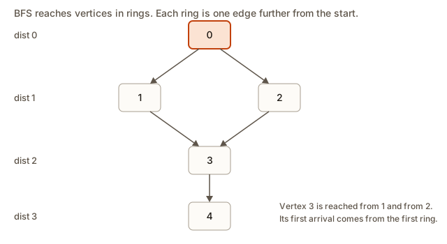 Five vertices arranged in rings by distance from vertex 0
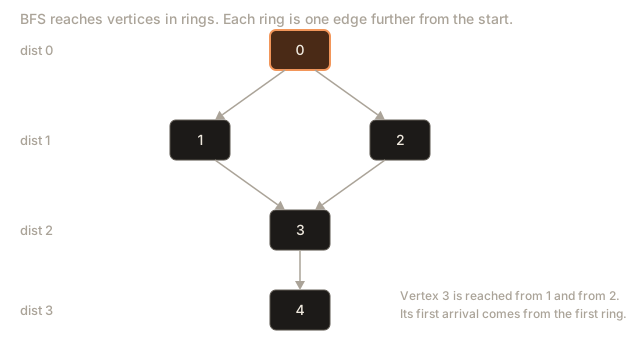
Vertex 3 has two neighbours in the first ring, 1 and 2. It is reached from 1 first only because 1 was popped before 2, which follows the order the edges were stored. Either way its distance is 2. The distance is the same no matter which neighbour reaches it first, because all of them are in the same ring.
Computing distances in C++
The second program runs BFS from a source it reads from input. The first line now holds n, m and the source s. The edges follow the same format as before.
Type this into the Input box:
6 5 0
0 1
0 2
1 3
2 3
3 4
The program prints:
dist[0] = 0
dist[1] = 1
dist[2] = 1
dist[3] = 2
dist[4] = 3
dist[5] = -1
Read the loop line by line. queue<int> q; creates an empty queue of vertex numbers. q.push(s) puts the source in it. The while loop keeps going as long as there is something to take out. q.front() looks at the vertex at the front and q.pop() removes it. Then the for loop checks each neighbour. The test dist[w] == -1 is the whole visited check: a neighbour with a distance has been reached already, so we skip it.
The distance for a new neighbour is dist[v] + 1. That is the core rule. If v is k edges from the source, then a neighbour of v that is not yet reached is k + 1 edges away at most, and BFS guarantees that this is exact.
The space cost is simple to read off the code. dist has n entries. The queue holds each vertex at most once, so it never holds more than n entries. The adjacency lists hold about e entries, counting both directions. The total is about n + e memory. Time is also about n + e: each vertex leaves the queue once, and each edge is checked a constant number of times. That is the standard answer to write in an interview: BFS on an adjacency list runs in O(n + e) time and O(n) extra space, not counting the graph itself.
Remembering the route
Distances tell you how far a vertex is. Often you need the route too. Suppose you want the path from 0 to 4 and not just the number 3. The trick is to store, for each vertex, the vertex it was reached from. That is called the parent. When BFS first reaches w from v, it sets parent[w] = v. Once the search finishes, you can walk backwards from the target through the parents until you reach the source. Reverse that list and you have the path.
The third program does exactly that. It also prints no path when the target cannot be reached, which is a case you must always handle.
Type this into the Input box for the first test. It asks for the path from 0 to 4 in the same graph:
6 5 0 4
0 1
0 2
1 3
2 3
3 4
The program prints:
distance: 3
path: 0 1 3 4
Now change the last number of the first line to 5, so the target is vertex 5, which has no edges. Keep the rest of the input the same. The program prints:
no pathTwo details matter. The loop that walks backwards stops when v becomes -1, which is the parent of the source. The source never gets a parent, because it was not reached from anything. The path is built backwards, so the program reverses it before printing. The walk also needs the dist[t] == -1 test first. Without it, the walk from an unreached vertex would stop at -1 immediately and print a meaningless one-vertex path.
Parents are how many real tools show a route. A map app that says "turn left, then right" is following the parent chain from the destination back to where you started.
Searching a grid
A grid, such as a map of a room or a game board, is a graph in disguise. Each open cell is a vertex. Two cells are neighbours when they touch up, down, left or right. You never need to build the adjacency list for a grid. Instead, when you visit a cell, you compute its neighbours by stepping in the four directions and checking that each step stays inside the grid and is not a wall.
The fourth program finds the fewest moves from the top-left cell to the bottom-right cell. A # is a wall and a . is open floor. The two arrays dr and dc hold the row and column changes for the four directions.
Type this into the Input box:
3 4
....
.##.
....
The program prints:
steps: 5Check it by hand. The grid has three rows and four columns. The top-left cell is (0,0) and the bottom-right is (2,3). One shortest route goes right along the top row to (0,3), down to (1,3), and down to (2,3). That is five moves. Five is the smallest possible answer here, because you must move down twice and right three times. The walls in the middle row only force the route to use the top row and the right column.
Now try a grid where the exit is cut off. Type this:
3 3
...
###
...
The program prints:
steps: -1The bottom row is unreachable because the middle row is all walls. The distance array keeps -1 for every cell in the bottom row, so the program prints -1 for the exit. Printing -1 is a common convention for "impossible", but you must say what it means in your answer to a user.
The grid version teaches a useful pattern. The queue holds pairs of numbers, queue<pair<int, int>>. Structured bindings, written auto [r, c] = q.front();, unpack the pair in one line. The direction arrays keep the four-way neighbour logic in one loop, so you do not repeat yourself four times.
A small warning. The program above assumes the top-left cell is open. If it is a wall, the search still starts from it, and the answer can be wrong. A careful solution checks the start and the goal first.
What the computer does with the memory
The matrix program below does no graph work. It only shows the cost of the matrix idea. It reads the number of vertices and prints how many bytes an adjacency matrix of int values would take.
Type this into the Input box:
100000The program prints:
matrix bytes: 40000000000That is about 40 gigabytes for one table of int values. A typical laptop has 8 to 16 gigabytes of memory. So the matrix is not an option for this graph, but the list is: 100,000 vertices and a few hundred thousand edges fit in a few megabytes.
Two details are easy to miss. First, the program uses long long for n. If it used int, the product n * n would overflow, because the largest int is about 2.1 billion. Second, sizeof(int) is 4 on most systems, but a C++ program should ask for it rather than assume it. Those two habits, using a wide enough type and not hard-coding sizes, prevent many bugs in graph code.
Why a queue and not a stack
Replace the queue with a stack and the code looks almost the same. A stack is last in, first out. You push and pop at the same end, like a pile of plates where you always take the top plate. Many students make this swap by accident. The program still runs and still prints numbers, so the mistake is easy to miss. That is why it is worth tracing the swap by hand once.
Use a graph with five vertices and these undirected edges: 0-1, 0-2, 1-3, 2-4 and 3-4. Written as lists in input order, the neighbours are: 0 has 1, 2; 1 has 0, 3; 2 has 0, 4; 3 has 1, 4; 4 has 2, 3. The correct distance from 0 to 3 is 2, through 1.
Trace the stack version. The stack starts as [0] and dist[0] is 0.
Pop 0. Its neighbours 1 and 2 get distance 1, and both are pushed. Stack [1, 2].
Pop 2, the last item pushed. Its neighbour 4 gets distance 2 and is pushed. Stack [1, 4].
Pop 4. Its neighbour 3 is new, so it gets distance dist[4] + 1, which is 3, and it is pushed. Stack [1, 3].
Pop 3 and then 1. Nothing new is found. The final distances are 0 1 1 3 2, so dist[3] is 3. That is wrong.
Now trace the queue version of the same graph. The queue starts as [0].
Pop 0. Push 1 and 2 with distance 1. Queue [1, 2].
Pop 1. Its neighbour 3 is new, so it gets distance 2 and is pushed. Queue [2, 3].
Pop 2. Its neighbour 4 is new, so it gets distance 2 and is pushed. Queue [3, 4].
Pop 3 and then 4. Nothing new. The final distances are 0 1 1 2 2, and dist[3] is 2. That is correct.
The difference is the order of the visits. The stack went deep first: 0, then 2, then 4, and only then came back to 1. By the time it reached 3 through 4, it had given 3 a long route, and it never went back to fix it. The queue finished the whole first ring, including 1, before it looked at anything in the second ring. So 3 was reached through 1 first, at the right distance.
The rule is simple. BFS needs the ring order, and only a queue keeps it. If your problem needs the search to go as deep as it can before backing up, use a stack or recursion instead. That is depth-first search, and the next lesson covers it.
Edge cases to check before you submit
Real tests try the cases that break careless code. Check each of these before you trust a graph program.
- Source equals target. The distance is 0 and the path is just the one vertex. The path loop in the third program handles this, because
parentof the source is-1. - No edges at all. Only the source is reached. Every other entry of
diststays-1. Make sure your code does not assume the graph has edges. - A single vertex. With
n = 1the lists have one entry each, and the BFS loop runs once and stops. - A self-loop, an edge from a vertex to itself. It is stored in that vertex's list. BFS is safe with it, because the neighbour already has a distance. Cycle checks in the next lesson must handle it with care.
- Duplicate edges, the same pair listed twice. They are harmless for BFS, but they make the degree count and the memory bigger.
- A disconnected graph. Vertices in other parts of the graph keep distance
-1. Decide in advance whether your output should say so. - A blocked start or exit in a grid. If the start cell is a wall, the answer is usually
-1, but the program above does not check. Add that check before you submit. - Several test cases in one input. Clear the lists and the arrays before the next case. Forgetting to do so is one of the most common reasons a second test case gives a strange answer.
Explaining BFS in an interview
Interviewers want to hear the idea before the code. A good short answer goes like this. "I put the source in a queue and mark it with distance 0. Each time I pop a vertex, I look at its neighbours. Any neighbour I have not reached gets the distance of the popped vertex plus one, and I push it. I mark a vertex when I push it, so each vertex is queued once. Each vertex is popped once and each edge is looked at a constant number of times, so the time is proportional to the vertices plus the edges."
Then say why it finds the fewest edges. The rings grow one step at a time, and the queue keeps them in order. If you mention that the stack version gives wrong distances, you show that you understand why the queue is the key part, not just the loop.
Common mistakes
The first mistake is forgetting the header for queue. If you write a BFS and leave out #include <queue>, g++ reports an error like this:
main.cpp: In function ‘int main()’:
main.cpp:5:5: error: ‘queue’ was not declared in this scope
    5 |     queue<int> q;
      |     ^~~~~
main.cpp:3:1: note: ‘std::queue’ is defined in header ‘<queue>’; this is probably fixable by adding ‘#include <queue>’
The fix is the line the note suggests. Read the note; it names the header. The next error in a longer output, expected primary-expression before ‘int’, is a follow-on error. It appears only because the first error left the compiler unsure what queue means. Fix the first error and the second usually disappears.
The second mistake is marking a vertex as visited when it leaves the queue, not when it enters. Consider this version of the inner loop:
for (int w : adj[v]) {
    if (dist[w] == -1) q.push(w);   // not marked yet!
}
Vertex 3 in our example is adjacent to both 1 and 2. When 1 is popped, 3 is still unmarked, so it is pushed. When 2 is popped before 3 leaves the queue, 3 is still unmarked again, so it is pushed a second time. The vertex is now queued twice. In a dense graph the same vertex can be queued many times, and the queue can grow far past n entries. Mark when you push, as the real program does.
The third mistake is using a matrix for a graph with a large number of vertices. The matrix program showed the cost: 100,000 vertices need about 40 gigabytes. If your program allocates vector<vector<int>> m(n, vector<int>(n)) for n equal to 100,000, the allocation fails with std::bad_alloc or the operating system kills the process. You will not see the matrix's cost in small tests, so check the size limits in the problem statement before you choose.
The fourth mistake is reading an undirected edge in only one direction. If the input says 0 1 is an edge and you only write adj[0].push_back(1), then BFS from 1 cannot reach 0. The fix is to add both directions, unless the problem says the graph is directed.
The fifth mistake is thinking that BFS distances count weights. They count edges. If each road has a length, BFS still counts roads, not kilometres. The next lessons handle weights.
A debugging walkthrough
Suppose a classmate writes the BFS but the answer for dist[4] is 4, not 3. What do you do?
Start with the small input. The graph has five edges, and you know the correct distances. Print the queue at each step. Add a line like this inside the while loop, before the pop:
cerr << "pop " << q.front() << " dist " << dist[q.front()] << "\n";Use cerr for debug lines, because it writes to a different stream from cout and is easy to remove later. Run with the sample. You might see pop 3 dist 2 followed by pop 4 dist 3, which is right. If you see dist 4, the bug is either the source being wrong or an extra edge. Check the input: maybe the file has an edge 4 3 that you did not expect, and maybe the program read m as 6, not 5. Printing m and each edge as you read it finds this in a minute.
The lesson is general. When a graph answer is wrong, check the graph first. Print the adjacency lists and compare them with the picture you drew. Most graph bugs are input bugs, not algorithm bugs.
Patterns that come up in interviews
BFS on an unweighted graph is the answer to "fewest steps" questions. Look for phrases like minimum moves, fewest hops, shortest transformation, or minimum number of rounds where each round moves one step in every direction. A grid with walls, a word that changes one letter at a time, and a set of rooms that light up each second all reduce to BFS.
Multi-source BFS is a variation. You push several starting cells into the queue at once, all with distance 0. The rings then spread from every source together. One example: for each empty cell, find the distance to the nearest fire. You do not run BFS once per cell. You run it once with all fires in the queue. This is much faster and it is a common interview point.
When the question asks for the number of ways rather than the shortest path, BFS still helps, but you must add counts. This is a step toward dynamic programming, which the module on that topic covers.
Practice
-
Change the neighbour list program so that it also prints each vertex's degree after its list. Hint: the degree is
adj[v].size(). Expected output for the sample input:0: 1 2 (degree 2)on the first line. -
Change the BFS distance program so that it prints the vertices in the order BFS first reaches them. Hint: push vertices into a
vectorthe first timedistis set, and print thatvectorat the end. -
Count how many vertices are exactly two edges from the source
0in the sample graph. Hint: count the entries withdist[v] == 2. -
Make the BFS distance program print
unreachableinstead of-1for vertices with no path. Make sure the vertex5line in the sample then readsdist[5] = unreachable. -
Write a grid BFS that starts from the top-left cell and finds the fewest steps to any cell in the last row, not just the bottom-right corner. Hint: stop as soon as you pop a cell whose row equals
R - 1. -
Given a grid with some
#walls, count how many open cells can be reached from the top-left cell. Hint: count the cells withdist != -1after the search. -
Estimate the memory for an adjacency list of 100,000 vertices and 300,000 undirected edges, storing each
intas 4 bytes. Hint: each edge is stored twice, and eachvectorhas a fixed overhead of about 24 bytes on a 64-bit system, so count both. -
Prove that a path found by BFS to a vertex has the fewest edges. Hint: assume a shorter path exists, look at the first ring where the two routes differ, and show that BFS would have reached the vertex from that ring earlier.
-
Explain in words why the program using
q.push(w)only whendist[w] == -1can never queue the same vertex twice, while the wrong version can. -
Change the grid program so that
#cells are allowed to be passed through at a cost of 1 extra step each. Hint: this is no longer an unweighted problem, so think about what must change in the queue. You will need the next lesson's tools.
Solution
-
Add
cout << " (degree " << adj[v].size() << ")";before the newline. For the sample input the first line becomes0: 1 2 (degree 2). -
Keep a
vector<int> order;. Right afterdist[w] = dist[v] + 1;, addorder.push_back(w);. Start withorder.push_back(s);before the loop. Printorderat the end. For the sample the order is0 1 2 3 4. -
Loop over
distand count the entries equal to 2. For the sample, vertices3has distance 2, so the answer is 1. Vertex3is the only one at distance 2. -
Replace the output line with
if (dist[v] == -1) cout << "unreachable"; else cout << dist[v];inside the loop, then add the newline. Vertex5then printsdist[5] = unreachable. -
Run the same BFS but stop when the popped cell's row is
R - 1. The first such cell popped has the fewest steps, so print its distance and exit. Print-1if the queue empties first. -
After the BFS, count every cell where
dist[r][c] != -1. That is the number of open cells reachable from the start, including the start itself. -
There are 300,000 edges, so 600,000 list entries at 4 bytes each is about 2.4 MB. Add 100,000 vectors at about 24 bytes each for the headers, which is about 2.4 MB more. The total is around 5 MB, which is tiny compared with the 40 GB matrix.
-
Suppose a shorter path exists to vertex
tthan the BFS path. Find the first vertex on the shorter path that the BFS reached at a larger distance than the shorter path gives. Its predecessor on the shorter path was reached correctly, by induction, so BFS would have reached it from that predecessor earlier. This contradicts the first arrival being late. -
A vertex gets a distance exactly once, at its first push, because the test
dist[w] == -1fails for every later neighbour. The wrong version does not set the distance at the push, so the test passes again for later neighbours, and the same vertex is pushed again. -
Once a wall costs extra, edges no longer all count the same. Plain BFS can give the wrong answer. You need Dijkstra's algorithm, which the next lesson introduces.
What you now know
- A graph is vertices plus edges. A directed edge has one direction, an undirected edge works both ways, and a weighted edge carries a number.
- An adjacency list stores
npluseentries and is the default. An adjacency matrix costsntimesncells and only pays off for dense graphs. - BFS uses a queue to visit vertices in rings. The first time a vertex is reached, its distance is the fewest edges from the source.
- Mark a vertex when you push it, not when you pop it, so it is queued only once.
- A parent array lets you rebuild the path, and it needs a check that the target was reached.
- A grid is a graph. Compute the four neighbours on the fly with direction arrays.
- BFS runs in
O(n + e)time andO(n)extra space on an adjacency list.